Hyperbolic frequency-modulated bat calls using hyperbolic scale transform and PHS HFM Sonar

The estimated IFs obtained by FRFT. (a) Eighth bat call. (b) Ninth bat call.

Summary of HFM Advantages and Disadvantages

Here are some key advantages and disadvantages of using hyperbolic frequency modulation (HFM) signals for sonar:

Advantages:

1. Doppler invariance - HFM signals have inherent Doppler invariant characteristics, making them well-suited for detecting moving targets.
2. Tolerant to moving targets - HFM can still produce peaks after matched filtering even at high target speeds, unlike linear FM signals.
3. Can use different frequency bands - HFM signals of different frequency bands can be combined in a pulse sequence, helping overcome propagation loss issues in certain frequency bands.
4. Improved accuracy - Using multiple HFM signals allows for mutual calculation of speed and distance, reducing errors compared to single signal calculations.
5. Suitable for coherent integration - The phase information can be preserved for coherent integration across pulse sequences, improving signal-to-noise ratio.

Disadvantages:

1. Complex processing - Requires more complex signal processing compared to simpler waveforms like continuous wave signals.
2. Coupling of velocity and distance - The ambiguity function of HFM has a "blade" shape, coupling velocity and distance measurements.
3. Time delay issues - Doppler shifts cause time delays after matched filtering, making ranging difficult with a single HFM pulse.
4. Frequency band limitations - A single HFM signal may have too much transmission loss in certain frequency bands of the underwater channel.
5. SNR requirements - Low SNR can still lead to errors in arrival time estimation and peak detection.
6. Computational complexity - Processing multiple HFM signals in a sequence increases the computational requirements.

In summary, while HFM offers significant advantages for sonar, especially for moving target detection, it also comes with increased complexity in signal design and processing. The use of HFM pulse sequences helps mitigate some single-pulse limitations but requires more sophisticated systems. 

Bat Sonar

Bats use hyperbolic frequency modulated (HFM) sonar in several sophisticated ways:

1. Echolocation: Bats emit HFM calls and use the echoes to navigate and locate prey. The document mentions that echolocating bats have acquired capabilities through evolution that are more intelligent and efficient than existing synthetic systems.

2. Waveform variation: Bats vary their waveforms during different phases of prey pursuit - searching, approaching, and capturing. This allows them to optimize their sonar for each stage of hunting.

3. Multiple harmonics: Bat calls often contain multiple harmonics with large energy differences. This may help them gather more information about their environment and targets.

4. Doppler compensation: Some bats, like the hipposiderid bat, can precisely compensate for Doppler shifts in their calls. This helps them accurately detect moving prey.

5. Clutter suppression: Bats use echo harmonic structure to distinguish their targets from background clutter.

6. Target recognition: The document suggests bats may use trends in call parameters for species identification of prey.

7. Ranging accuracy: Bats appear to adjust their call parameters (like decreasing intra-pulse delay) to improve ranging accuracy as they approach prey.

8. Adaptive beam steering: Some bats, like Egyptian fruit bats, can control their sonar beam direction by adjusting their tongues, similar to phased array radar.

9. Wideband signals: Bat calls are often wideband FM signals, which can provide more information about targets than narrowband signals.

10. Optimal Doppler tolerance: The HFM waveforms used by bats are thought to be optimized for Doppler tolerance, allowing them to detect prey moving at various speeds.

The document emphasizes that bat sonar capabilities have evolved over millions of years and are in many ways superior to human-made sonar systems. Researchers are studying bat sonar to improve biomimetic technologies and synthetic echolocation systems. 

PHS Sonar

PHS (Pulse sequence method based on Hyperbolic Frequency Modulation) sonar is an approach described in the document that aims to improve speed measurement and ranging accuracy using multiple HFM signals. Here's a breakdown of how it works and how it compares to bat sonar:

How PHS uses HFM:

1. Multiple HFM signals: PHS uses a sequence of HFM signals with different frequency bands and pulse widths.

2. Velocity measurement: It calculates target velocity by comparing the time delays between different HFM signals after matched filtering.

3. Ranging: PHS uses the relationships between multiple HFM echoes to improve ranging accuracy.

4. Coherent integration: It allows for coherent integration across pulse sequences to improve signal-to-noise ratio.

5. Adaptability: By using multiple frequency bands, PHS can overcome issues with excessive propagation loss in certain frequency ranges.

Comparison to bat sonar:

Similarities:
1. Use of HFM: Both PHS and bat sonar utilize HFM signals for their Doppler invariant properties.
2. Multiple frequency bands: Bats use multiple harmonics, while PHS uses different frequency bands across pulses.
3. Adaptability: Both systems can adapt to different environmental conditions and target scenarios.

Differences:
1. Complexity: Bat sonar is likely more sophisticated, having evolved over millions of years.
2. Real-time processing: Bats process sonar information in real-time with highly evolved neural systems, while PHS relies on digital signal processing.
3. Emission control: Bats can dynamically control their call emissions, including beam steering, which isn't mentioned as a feature of PHS.
4. Bandwidth: Bat calls often cover a wider frequency range than typical PHS implementations.
5. Integration with other senses: Bats integrate sonar with other sensory inputs, which PHS doesn't do.

Advantages of PHS over single HFM:
1. Improved accuracy: PHS can achieve better ranging and speed measurement accuracy than single HFM signals.
2. Resilience to channel effects: Using multiple frequency bands helps overcome issues with propagation loss in specific frequencies.
3. Flexibility: PHS can be adjusted for different scenarios by changing the HFM signal parameters in the sequence.

While PHS represents an advancement in synthetic sonar systems using HFM, it still doesn't match the full capabilities and adaptability of bat sonar. However, it demonstrates how principles observed in bat echolocation can be applied to improve human-made sonar systems.

Parameter estimation of the hyperbolic frequency-modulated bat calls using hyperbolic scale transform | The Journal of the Acoustical Society of America | AIP Publishing

pubs.aip.org 

 

Zhang, Liang, Du, Qinglei

---

July 01 2024

Liang Zhang; Department of Early Warning Technology, Air Force Early Warning Academy, Wuhan, 430019, China

Qinglei Du; Department of Early Warning Technology, Air Force Early Warning Academy, Wuhan,  30019, China

J. Acoust. Soc. Am. 156, 16–28 (2024)

Echolocating bats are known to vary their waveforms at the phases of searching, approaching, and capturing the prey. It is meaningful to estimate the parameters of the calls for bat species identification and the technological improvements of the synthetic systems, such as radar and sonar. The type of bat calls is species-related, and many calls can be modeled as hyperbolic frequency- modulated (HFM) signals. To obtain the parameters of the HFM-modeled bat calls, a reversible integral transform, i.e., hyperbolic scale transform (HST), is proposed to transform a call into two-dimensional peaks in the “delay-scale” domain, based on which harmonic separation and parameter estimation are realized. Compared with the methods based on time-frequency analysis, the HST-based method does not need to extract the instantaneous frequency of the bat calls, only searching for peaks. The verification results show that the HST is suitable for analyzing the HFM-modeled bat calls containing multiple harmonics with a large energy difference, and the estimated parameters imply that the use of the waveforms from the searching phase to the capturing phase is beneficial to reduce the ranging bias, and the trends in parameters may be useful for bat species identification.

I. INTRODUCTION

Bats are well known for their echolocation, like that used in radar and sonar.¹ For example, bats also use transmitted beams,² and the direction can be controlled by moving their head or changing the shape of the mouth or nose. “Advanced” Egyptian fruit bats change the beams by adjusting their tongues,³ similar to the phased array radar. In addition, some issues, such as Doppler compensation,⁴ clutter suppression,⁵ target recognition,⁶ and countermeasures^7,8 are important for both the bats and the synthetic systems. Through over 50 × 10⁶ years of evolution,^9,10 the echolocating bats acquired the capabilities, which actually are more intelligent and efficient than the existing synthetic systems.¹¹ Previous studies have shown that bats vary the waveform during the phases of searching, approaching, and capturing the prey.^12,13 These waveforms are all frequency modulated (FM),^14,15 and many are accurately referred to as the hyperbolic frequency modulated (HFM) signals.^12,16,17 A question naturally arises: “What exactly are the parameters of these waveforms, and how do they change?” This is an interesting but rarely studied subject. This article aims to obtain the parameters of the HFM-modeled bat calls, and explain the waveform strategy from the perspective of correlation detection used in radar and sonar, which may be significant for bat species identification¹⁸ and the design of biomimetic systems.^19,20

To obtain the parameters of HFM-modeled bat calls, it is easy to think of using the existing methods for estimating HFM signal, such as the methods based on group delay (GD) fitting^21,22 and those based on instantaneous frequency (IF) fitting.^23,24 However, the bat calls usually contain multiple harmonics, but GD-based methods require extracting the GD of each component from the spectrum, which is not feasible. In addition, there is a large energy difference between the harmonics, but IF-based methods need to extract the IF of each component from the time-frequency distribution (TFD) of the signal, which is not easy to implement unless a “clean” approach is taken to separate each component,²⁵ just as is done in this paper. Finally, the number of the bat calls may be large, and the estimating process needs to be as simple as possible, for example, the method in this paper only needs a peak search on the proposed hyperbolic scale transform (HST) of a bat call pulse. HST is a linear and reversible transform, capable of transforming an HFM-modeled bat call into several peaks in the “delay-scale” domain and obtaining harmonic parameters according to the peak position. The “delay” above consists of two parts: the first is the time delay of a bat call pulse in the recorded data, and the second is related to a characteristic of the HFM signal, and determined by the model parameters. Of course, if the bat call pulse has been extracted, the first part will be zero. In addition, as a signal processing tool, the proposed HST is not only suitable for the application in this paper but can be used in other fields involving HFM signal processing, such as interference suppression in sonar,²⁶ direction of arrival estimation of wideband signal,²⁷ and so on.

The remainder of the paper is structured as follows. The signal models of the bat call with multiple harmonics are introduced in Sec. II. The HST is proposed in Sec. III, including mathematical definition, property, implementation, and computational complexity. HST-based parameter estimation flow is given in Sec. IV. The performance of HST is validated and discussed using three bat call datasets in Sec. V. A conclusion is drawn in Sec. VI.

II. BAT CALL SIGNAL

To find the optimal Doppler tolerant waveforms, the HFM model is derived in Ref. 16 and found to be used by some bats, such as the long-tailed bat²⁸ and the big brown bat.²⁹ 

A. Model

Considering a $N$-components HFM signal with duration $T$⁠, chirp rate $k_n$⁠, and starting frequency $f_{1,n}$ for the $n$th component $s_n(t)$⁠, the multi-harmonic bat call can be modeled as

$x\left(t\right)=w\left(t\right)\sum _{n=1}^N{A}_n{s}_n\left(t\right)=w\left(t\right)\sum _{n=1}^N{A}_n{\mathrm{e}}^{\mathrm{i}2\pi (1/k_n)\text{ln}\hspace{0.17em}\left[1+k_n{f}_{1,n}t\right]},$(1)

where $t$ is time, $t\in [0,T]$⁠, $w(t)$ is pulse envelope, $N$ is harmonic number, $A_n$ is the amplitude of the $n$th harmonic, $A_1>A_2>\cdots >A_N$⁠, and

where $f_{2,n}$ is the ending frequency, $f_{2,n}<f_{1,n}$⁠, implying a down-sweeping mode. Now, taking the derivative of the phase in Eq. (1) yields the IF of the $n$th harmonic as

which can be expressed as

It can be seen that the IF is a delayed version of $(1/k_n)/t$ with the delay $1/(k_n{f}_{1,n})$⁠. To distinguish the delay of a call pulse in the recorded audio data, $1/(k_n{f}_{1,n})$ is named the intra-pulse delay (IPD) of $n$th harmonic in this paper. The existence of the characteristic is reasonable because $1/(k_{n}t)$ will approach infinity when $t\to 0$⁠, representing a physically impossible signal. The definition of IPD is meaningful because it will affect the ranging bias, if bats adopt correlation detection in the synthetic echolocating systems, which will be illustrated later by analyzing three feeding buzzes. At present, some studies also consider modeling the bat calls, especially the buzz phase calls, as linear frequency modeled (LFM) signals.²⁵ The HFM-modeled bat call signal is closely related to the LFM signal,³⁰ more precisely, the quadratic frequency modulated signal, because the third-order Maclaurin series approximation to the phase of the $n$th harmonic in Eq. (1) is

${\varphi }_n\left(t\right)=2\pi \frac{1}{k_n}\text{ln}\hspace{0.17em}\left[1+k_n{f}_{1,n}t\right]\approx 2\pi [f_{1,n}t-\frac{1}{2}\frac{B_n\left(1-{\xi }_n/2\right)}{T\left(1+{\xi }_n/2\right)}{t}^2-\frac{1}{3}{\xi }_n\frac{B_n\left(1-{\xi }_n/2\right)}{T^2{\left(1+{\xi }_n/2\right)}^2}{t}^3],$

(5)

where $B_n$ is the harmonic bandwidth, $B_n=f_{1,n}-f_{2,n}$⁠, and ${\xi }_n$ is the ratio of the bandwidth to center frequency. When ${\xi }_n$ is small, the third term in the brackets of Eq. (5) can be discarded, then the HFM-modeled bat call degenerates into a LFM-modeled bat call of

$x\left(t\right)=w\left(t\right)\sum _{n=1}^N{A}_n{\mathrm{e}}^{\mathrm{i}2\pi f_{1,n}t}{\mathrm{e}}^{\mathrm{i}\pi {\rho }_n{t}^2},$

(6)

with the starting frequency $f_{1,n}$ and linear chirp rate ${\rho }_n$ of

${\rho }_n=-\frac{B_n\left(1-{\xi }_n/2\right)}{T\left(1+{\xi }_n/2\right)}=-f_{2,n}^2{k}_n,\hspace{1em}{\rho }_n<0.$

(7)

The chirp rate $k_n$ in the HFM model is different from the linear chirp rate ${\rho }_n$ in the LFM model, because $k_n$ has no dimension, while ${\rho }_n$ is usually MHz/s. Because of this, $k_n$ is also named as the modulation index or period slope in some studies.^23,24

B. Spectrum

Different from the waveforms in radar and sonar, there is a modulation in the envelope of the bat call pulse and a solution of the weighted $p$th-order Bessel function leads to the optimal Doppler tolerance.¹⁶ Assuming that $w(t)$ is a rectangular window, the principle of stationary phase can be used to obtain the spectrum of the HFM component $s_n(t)$ of

$S_n\left(f\right)\approx \frac{1}{\sqrt{k_n}}\frac{1}{f}{\mathrm{e}}^{\mathrm{i}2\pi (1/k_n{f}_{1,n})f}{\mathrm{e}}^{\mathrm{i}2\pi (1/k_n)\text{ln}\hspace{0.17em}(f_{1,n}/f)},\hspace{1em}f>0,$

(8)

which is derived in  Appendix A. Then, using the property of the linearity of Fourier transform, the spectrum of the bat call pulse in Eq. (1) is obtained by

$X\left(f\right)=\sum _{n=1}^N{A}_n{S}_n\left(f\right)\approx \sum _{n=1}^N{A}_n\frac{1}{\sqrt{k_n}}\frac{1}{f}{\mathrm{e}}^{\mathrm{i}2\pi (1/k_n{f}_{1,n})f}{\mathrm{e}}^{\mathrm{i}2\pi (1/k_n)\text{ln}\hspace{0.17em}\left(f_{1,n}/f\right)},$

(9)

where the first complex exponent is related to the IPD of $1/(k_n{f}_{1,n})$ and the second is an analytic form of a sine wave about the logarithmic frequency with “frequency” of $1/k_n$⁠. In the following, HST will be designed to compensate for the two terms.

III. HYPERBOLIC SCALE TRANSFORM

If the spectrum in Eq. (9) is considered as a time series, the parameters of the bat call pulse can be obtained by searching the IPD and estimating the “frequency” of the series with “logarithmic time.” Based on the idea, HST is designed below.

A. Mathematical definition

According to the analysis above, the HST of a continuous signal $x(t)$ is defined as

$\begin{array}{c}\text{HST}\left[x\left(t\right)\right]=H_X\left(\tau ,c\right)={\int }_0^{\infty }X\left(f\right){\Upsilon }_{\tau }\left(c,f\right)\mathrm{d}f={\int }_0^{\infty }X\left(f\right)\frac{1}{\sqrt{f}}{\mathrm{e}}^{-\mathrm{i}2\pi f\tau }{\mathrm{e}}^{-\mathrm{i}2\pi c\hspace{0.17em}\text{ln}\hspace{0.17em}f}\mathrm{d}f,\end{array}$

(10)

where HST[·] denotes the HST, $\tau$ is delay, $c$ is scale, a physical attribute like frequency, $X(f)$ is the spectrum of $x(t)$⁠, and ${\Upsilon }_{\tau }(c,f)$ is the kernel functions given by

${\Upsilon }_{\tau }\left(c,f\right)=\frac{1}{\sqrt{f}}{\mathrm{e}}^{-\mathrm{i}2\pi f\tau }{\mathrm{e}}^{-\mathrm{i}2\pi c\hspace{0.17em}\text{ln}\hspace{0.17em}f},$

(11)

in which the first term is used to ensure orthogonality of ${\Upsilon }_{\tau }(c,f)$ about $c$⁠, and the last two terms are designed to match the spectrum in Eq. (9). ${\Upsilon }_{\tau }(c,f)$ satisfy the following relations:

${\int }_{-\infty }^{\infty }{\int }_0^{\infty }{\gamma }_{\tau }^{\ast }\left(c^{\prime },f\right){\gamma }_{\tau }\left(c,f\right)\mathrm{d}f\mathrm{d}\tau =\delta \left(c^{\prime }-c\right),$(12)

${\int }_{-\infty }^{\infty }{\int }_{-\infty }^{\infty }{\gamma }_{\tau }^{\ast }\left(c,f^{\prime }\right){\gamma }_{\tau }\left(c,f\right)\mathrm{d}c\mathrm{d}\tau =\delta \left(f^{\prime }-f\right),$(13)

${\int }_0^{\infty }{\int }_{-\infty }^{\infty }{\gamma }_{{\tau }^{\prime }}^{\ast }\left(c,f\right){\gamma }_{\tau }\left(c,f\right)\mathrm{d}c\mathrm{d}f\ne \delta \left(\tau -{\tau }^{\prime }\right),$(14)

which is derived in  Appendix B. It can be seen that ${\Upsilon }_{\tau }(c,f)$ is not orthogonal about $\tau$⁠, meaning that if the bat call can be transformed into peaks in HST image, the peaks will be a little wider in the delay dimension. The expression of HST is similar to that of scale transform (ST),³¹ a restriction of the $\beta -$ Mellin transform with $\beta =0.5$⁠, and the HST of $x(t)$ is actually the ST of $X(f){\mathrm{e}}^{-\mathrm{i}2\pi f\tau }$⁠. Since ST is reversible, the inverse HST is defined as

$\begin{array}{c}\text{IHST}\left[H_X\left(\tau ,c\right)\right]=X_{\tau }\left(f\right)={\int }_{-\infty }^{\infty }{H}_X\left(\tau ,c\right){\Upsilon }_{\tau }^{\ast }\left(c,f\right)\mathrm{d}c={\int }_{-\infty }^{\infty }{H}_X\left(\tau ,c\right)\frac{1}{\sqrt{f}}{\mathrm{e}}^{\mathrm{i}2\pi f\tau }{\mathrm{e}}^{\mathrm{i}2\pi c\hspace{0.17em}\text{ln}\hspace{0.17em}f}\mathrm{d}c,\end{array}$(15)

where IHST[·] denotes the inverse hyperbolic scale transform, which is the inverse ST of $H_X(\tau ,c){\mathrm{e}}^{\mathrm{i}2\pi f\tau }$⁠. Owing to the orthogonality of ${\Upsilon }_{\tau }(c,f)$ about $c$ and $f$⁠, we can perform scale filtering at a certain $\tau$ and a following inverse Fourier transform leads to the desired time-domain signal. It should be noted that HST also has a certain similarity to the Fourier Mellin transform, commonly used in image processing,³² both calculating the ST of the signal spectrum. However, the phase of the spectrum is retained and modulated in HST, while its modulus is taken in the Fourier Mellin transform to eliminate the delay effect, more conducive to extract the scale-invariant features of the images.³³ 

B. Property analysis

As can be seen from the above analysis, the HST is linear and reversible. To analyze the other properties, the substitution of $x=\text{ln}\hspace{0.17em}f$ into Eq. (10) yields

$H_X\left(\tau ,c\right)={\int }_{-\infty }^{\infty }\sqrt{{\mathrm{e}}^x}X\left({\mathrm{e}}^x\right){\mathrm{e}}^{-\mathrm{i}2{\pi \mathrm{e}}^x\tau }{\mathrm{e}}^{-\mathrm{i}2\pi cx}\mathrm{d}x=F\left[\sqrt{{\mathrm{e}}^x}X\left({\mathrm{e}}^x\right){\mathrm{e}}^{-\mathrm{i}2{\pi \mathrm{e}}^x\tau }\right],$(16)

where F[·] denotes the Fourier transform. The above formula illustrates the relationship between the proposed HST and Fourier transform. Now, according to the properties of Fourier transform, three covariance properties of HST are derived below.

• P1: Time-shift covariance

  $y\left(t\right)=x\left(t-{\tau }_0\right)\Rightarrow Y\left(f\right)=X\left(f\right){\mathrm{e}}^{-\mathrm{i}2\pi f{\tau }_0}\Rightarrow H_Y\left(\tau ,c\right)=H_X\left(\tau +{\tau }_0,c\right).$(17)

  Proof: Let $Y(f)=X(f){\mathrm{e}}^{-\mathrm{i}2\pi f{\tau }_0}$⁠, substituting it into Eq. (16) yields

  $H_Y\left(\tau ,c\right)=F\left[{\mathrm{e}}^{-\mathrm{i}2{\pi \mathrm{e}}^x\left(\tau +{\tau }_0\right)}X\left({\mathrm{e}}^x\right)\sqrt{{\mathrm{e}}^x}\right]=H_X\left(\tau +{\tau }_0,c\right).$(18)

• P2: Time-scaling covariance

  $y\left(t\right)=\sqrt{\beta }x\left(\beta t\right)\Rightarrow Y\left(f\right)=\frac{1}{\sqrt{\beta }}X\left(\frac{f}{\beta }\right)\Rightarrow H_Y\left(\tau ,c\right)={\mathrm{e}}^{-\mathrm{i}2\pi c\hspace{0.17em}\text{ln}\hspace{0.17em}\beta }{H}_X\left(\beta \tau ,c\right).$(19)

  Proof: Let $Y(f)=X(f/\beta )/\sqrt{\beta }$⁠, $\beta >0$⁠, substituting it into Eq. (16) yields

  $\begin{array}{c}{H}_Y\left(\tau ,c\right)=F\left[{\mathrm{e}}^{-\mathrm{i}2{\pi \mathrm{e}}^x\tau }\frac{1}{\sqrt{\beta }}X\left(\frac{{\mathrm{e}}^x}{\beta }\right)\sqrt{{\mathrm{e}}^x}\right]=F\left[{\mathrm{e}}^{-\mathrm{i}2{\pi \mathrm{e}}^{x-\text{ln}\hspace{0.17em}\beta }\beta \tau }\frac{1}{\sqrt{\beta }}X\left({\mathrm{e}}^{x-\text{ln}\hspace{0.17em}\beta }\right)\sqrt{{\mathrm{e}}^{x-\text{ln}\hspace{0.17em}\beta }}\sqrt{{\mathrm{e}}^{\hspace{0.17em}\text{ln}\hspace{0.17em}\beta }}\right]=F\left[{\mathrm{e}}^{-\mathrm{i}2{\pi \mathrm{e}}^{x-\text{ln}\hspace{0.17em}\beta }\left(\beta \tau \right)}X\left({\mathrm{e}}^{x-\text{ln}\hspace{0.17em}\beta }\right)\sqrt{{\mathrm{e}}^{x-\text{ln}\hspace{0.17em}\beta }}\right]={\mathrm{e}}^{-\mathrm{i}2\pi c\hspace{0.17em}\text{ln}\hspace{0.17em}\beta }{H}_X\left(\beta \tau ,c\right).\end{array}$(20)

• P3: Hyperbolic time-shift covariance

  $Y\left(f\right)={\mathrm{e}}^{-\mathrm{i}2\pi c_0\hspace{0.17em}\text{ln}\hspace{0.17em}\left(f/f_1\right)}X\left(f\right)\Rightarrow H_Y\left(\tau ,c\right)={\mathrm{e}}^{\mathrm{i}2\pi c_0\hspace{0.17em}\text{ln}\hspace{0.17em}\left(f_1\right)}{H}_X\left(\tau ,c+c_0\right).$(21)

  Proof: Let $Y(f)=\text{exp}(-\mathrm{i}2\pi c_0\hspace{0.17em}\text{ln}\hspace{0.17em}(f/f_1))X(f)$⁠, substituting it into Eq. (16) yields

  $H_Y\left(\tau ,c\right)=F\left[{\mathrm{e}}^{-\mathrm{i}2{\pi \mathrm{e}}^x\tau }{\mathrm{e}}^{-\mathrm{i}2\pi c_0\hspace{0.17em}\text{ln}\hspace{0.17em}\left({\mathrm{e}}^x/f_1\right)}X\left({\mathrm{e}}^x\right)\sqrt{{\mathrm{e}}^x}\right]={\mathrm{e}}^{\mathrm{i}2\pi c_0\hspace{0.17em}\text{ln}\hspace{0.17em}\left(f_1\right)}{H}_X\left(\tau ,c+c_0\right).$(22)

Remark: The property of P1 is very useful for parameter estimation of bat call, because there may be a delay of the real bat call in the signal extracted from the noisy recordings,³⁴ but this does not affect the accurate estimation of chirp rate. In addition, if the sampling frequency is much greater than the signal bandwidth, the IPD search range can be narrowed by operating time scaling on the bat call pulse according to P2; however, the bat call datasets used in this paper are not the case.

C. Computational complexity

The HST of a continuous signal $x(t)$ is the ST of the modulated spectrum of $X(f){\mathrm{e}}^{-\mathrm{i}2\pi f\tau }$⁠, meaning that a fast numerical calculation can be obtained using fast ST,³⁵ which is equivalent to the description in Eq. (16). Because of the adoption of digital interpolation and fast Fourier transform, the computational complexity of the fast ST can be controlled to a low level of $O[L\hspace{0.17em}\text{ln}\hspace{0.17em}L]$⁠, where $L$ is exponential sample number. According to the exponential sampling theorem,³⁶  $L$ should be not less than $N\hspace{0.17em}\text{ln}\hspace{0.17em}N$⁠, $N$ is the uniform sample number. As to the HST, several times fast ST needs to be calculated for each $\tau$ with a computational complexity of $O[PL\hspace{0.17em}\text{ln}\hspace{0.17em}L]$⁠, where $P$ is the search number of the delay $\tau$ and $L$ is the exponential sample number of $X(f){\mathrm{e}}^{-\mathrm{i}2\pi f\tau }$⁠. Since $X(f){\mathrm{e}}^{-\mathrm{i}2\pi f\tau }$ is the spectrum of $x(t-\tau )$⁠, $L$ should also be not less than $N_1\hspace{0.17em}\text{ln}\hspace{0.17em}{N}_1$⁠, $N_1$ is the sample number of $x(t-\tau )$⁠. Assuming that $N_1$ is slightly larger than $N$⁠, the computational complexity of HST is exactly $O[P(N\hspace{0.17em}\text{ln}\hspace{0.17em}N)\hspace{0.17em}\text{ln}\hspace{0.17em}(N\hspace{0.17em}\text{ln}\hspace{0.17em}N)]$ with a consistent scale resolution of $1/\hspace{0.17em}\text{ln}\hspace{0.17em}{N}_1$⁠. As to the discretization of $\tau$⁠, the delay range and the delay step need to be determined, where the step can be set as a sampling period or more. A larger one implies a coarser delay search and a smaller one indicates a finer search. However, the setting of the delay range depends on the signal parameters. In Sec. IV, we will analyze the HST of the HFM-modeled bat call pulse and give a reasonable solution.

IV. PARAMETER ESTIMATION

Bat calls often contain several harmonics with large energy differences. It is difficult to obtain the parameters of each harmonic by calculating HST only once, because of the masking effect of strong harmonics on weak harmonics, so it is necessary to use inverse HST to filter out the strong harmonics before estimating the parameters of weak harmonics. Based on this idea, this section will give an estimation flow using HST and inverse HST, and demonstrate the advantages of the proposed method mathematically by analyzing the limitations of the existing estimation methods.

A. Proposed method

The design of the kernel functions in HST is to compensate for the exponent terms in the signal spectrum. Now, substituting Eq. (9) into Eq. (10) yields the HST of a bat call pulse as

where $H_{S_n}(\tau ,c)$ is the HST of the $n$th HFM component, and

$H_{S_n}\left(\tau ,c\right)=\left(\frac{1}{\sqrt{k_n}}{\mathrm{e}}^{\mathrm{i}2\pi (1/k_n)\text{ln}\hspace{0.17em}{f}_{1,n}}\right){\int }_{f_{1,n}}^{f_{2,n}}\frac{1}{\sqrt{f}}{\mathrm{e}}^{\mathrm{i}2\pi \left((1/k_n{f}_{1,n})-\tau \right)f}{\mathrm{e}}^{-\mathrm{i}2\pi \left((1/k_n)+c\right)\hspace{0.17em}\text{ln}\hspace{0.17em}f}\mathrm{d}\left(\text{ln}\hspace{0.17em}f\right)\approx \delta \left(\tau -\frac{1}{k_n{f}_{1,n}}\right)\delta \left(c+\frac{1}{k_n}\right),$(24)

which approximates a two-dimensional (2D) peak at the peak delay ${\tau }_{\mathrm{p}}$ and the peak scale $c_{\mathrm{p}}$ of

It can be seen that ${\tau }_{\mathrm{p}}$ is equal to the IPD of $n$th harmonics and $c_{\mathrm{p}}$ is related to the reciprocal of the chirp rate. In particular, when $\tau ={\tau }_{\mathrm{p}}$⁠, Eq. (24) can be approximated as

$H_{S_n}\left({\tau }_{\mathrm{p}},c\right)\approx \left(\frac{1}{\sqrt{k_n}}{\mathrm{e}}^{\mathrm{i}2\pi (1/k_n)\text{ln}\hspace{0.17em}{f}_{1,n}}\right)\hspace{0.17em}\text{ln}\hspace{0.17em}\left(\frac{f_{2,n}}{f_{1,n}}\right)\text{sinc}\left\{\pi \hspace{0.17em}\text{ln}\hspace{0.17em}\left(\frac{f_{2,n}}{f_{1,n}}\right)\left(c+1/k_n\right)\right\},$(26)

where sinc[·] denotes the sinc function. Then, the parameters of $n$th harmonic can be estimated by

There are two issues to be noted here. First, to ensure the presence of peaks in HST, the delay search range needs to cover all the intra-pulse delays (IPDs) of the harmonics. According to the expression of the chirp rate in Eq. (2), the peak delay ${\tau }_{\mathrm{p}}$ of $n$th harmonics can be exactly expressed as

${\tau }_{\mathrm{p}}=\frac{1}{k_n{f}_{1,n}}=T\frac{f_{2,n}}{f_{1,n}-f_{2,n}}.$(28)

Since most of the bat calls are down-sweeping, i.e., ${\tau }_{\mathrm{p}}>0$⁠, meaning that the minimum delay $d_{\text{min}}$ can be set to 0, but the maximum delay $d_{\text{max}}$ is not easy to determine, as ${\tau }_{\mathrm{p}}$ tends to infinity theoretically, if $f_{1,n}$ is close to $f_{2,n}$⁠. The situation usually does not happen, and an empirical setting of $d_{\text{max}}$ of three times the signal duration is sufficient. In addition, there is a large energy difference between the harmonics, resulting in a masking of the strong harmonics on the weak harmonics in the “delay-scale” domain, so it is necessary to estimate the parameters of the strongest harmonic first by searching the highest 2D peak in HST image of a bat call, according to Eq. (27), then with a “clean” approach to estimate the parameters of the sub-strong harmonic from the HST image of the signal after scale filtering, and so on. As to the bat call $x(t)$⁠, the filtered signal can be expressed as

$\begin{array}{c}\tilde{x}\left(t\right)=x\left(t\right)-F^{-1}\left\{\text{IHST}\left[\text{HST}\left[x\left(t\right)\right]\Gamma \left(c\right)\right]\right\}=x\left(t\right)-{\mathrm{F}}^{-1}\left\{{\text{ST}}^{-1}\left[\text{ST}\left[F\left[x\left(t\right)\right]{\mathrm{e}}^{-\mathrm{i}2\pi f{\tau }_{\mathrm{p}}};c\right]\Gamma \left(c\right);f\right]\right\},\end{array}$(29)

where F⁻¹[·], ST[·] and ST⁻¹[·] denote inverse Fourier transform, ST, and inverse ST, respectively, and $\Gamma (c)$ is a rectangular window with the center at $c_{\mathrm{p}}$ and width set to cover the main-lobe width of the sinc function in Eq. (26). As the analysis above, Table I shows the parameter estimation flow for the harmonics within a bat call pulse, where the bat call pulse is extracted from the recorded data, and the number of harmonics to be estimated is set by yourself. The reliability of this process is closely related to the extraction of effective pulses, which involves bat signal detection.³⁴ 

TABLE I.

HST and inverse HST are used to estimate the harmonic parameters of a bat call pulse.

Input: Bat call pulse $x(t)$⁠, minimum delay $d_{\text{min}}$⁠, maximum delay $d_{\text{max}}$⁠, and harmonic number $N$

1) Calculate Fourier transform of $x(t)$⁠, and get its spectrum $X(f)$⁠.

2) Calculate HST of $X(f)$⁠, and get $H_X(\tau ,c)$⁠, $\tau \in [d_{\text{min}},d_{\text{max}}]$⁠.

3) Search the maximum of $\left|H_X(\tau ,c)\right|$⁠, and obtain the peak delay ${\tau }_{\mathrm{p}}$ and the peak scale $c_{\mathrm{p}}$⁠.

4) Estimate the chirp rate $k_n$ and the starting frequency $f_{1,n}$ according to Eq. (27).

5) Filter out the strongest harmonic of $x(t)$ through Eq. (29), and get the filtered signal.

6) Repeat steps 1–5 until the parameters of $N$ harmonics have been estimated.

Output: The estimated chirp rate $k_n$ and starting frequency $f_{1,n}$⁠, $n=1,2,\dots ,N$

Input: Bat call pulse $x(t)$⁠, minimum delay $d_{\text{min}}$⁠, maximum delay $d_{\text{max}}$⁠, and harmonic number $N$

1) Calculate Fourier transform of $x(t)$⁠, and get its spectrum $X(f)$⁠.

2) Calculate HST of $X(f)$⁠, and get $H_X(\tau ,c)$⁠, $\tau \in [d_{\text{min}},d_{\text{max}}]$⁠.

3) Search the maximum of $\left|H_X(\tau ,c)\right|$⁠, and obtain the peak delay ${\tau }_{\mathrm{p}}$ and the peak scale $c_{\mathrm{p}}$⁠.

4) Estimate the chirp rate $k_n$ and the starting frequency $f_{1,n}$ according to Eq. (27).

5) Filter out the strongest harmonic of $x(t)$ through Eq. (29), and get the filtered signal.

6) Repeat steps 1–5 until the parameters of $N$ harmonics have been estimated.

Output: The estimated chirp rate $k_n$ and starting frequency $f_{1,n}$⁠, $n=1,2,\dots ,N$

B. Traditional estimation methods

Parameter estimation of the HFM-modeled bat calls can be considered a special case of HFM signal parameter estimation. As mentioned in Sec. I, the GD-based methods^21,22 for parameter estimation of the mono-component HFM signal are not feasible because the bat calls usually contain multiple harmonics, while the IF-based methods^23,24 seem to be feasible, but require more human assistance to obtain the IF of each harmonic, which is not suitable for a large number of bat calls. In addition, some studies try to use Q distribution and fractional Fourier transform (FRFT) for bat call analysis.^25,37 Below, we will analyze their feasibility for parameter estimation.

Q distribution, representing a signal in the “time-scale” domain, is used to analyze the scale domain characteristics of a bat pulse (Eptesicus focus), finding that there is a quadratic phase coupling between the harmonics.³⁷ The Q distribution of the continuous signal $x(t)$ is defined as

$Q_x\left(t,c\right)={\int }_0^{\infty }x\left(\sqrt{a}t\right)x^{\ast }\left(\frac{1}{\sqrt{a}}t\right)\frac{1}{a}{\mathrm{e}}^{-\mathrm{i}2\pi c\hspace{0.17em}\text{ln}\hspace{0.17em}a}\mathrm{d}a,$(30)

where $a$ is the time-scaling factor. It can be seen that the expression of Q distribution is also similar to that of the ST, with the relationship of

$Q_x\left(t,c\right)=\text{ST}\left[\frac{1}{\sqrt{a}}x\left(\sqrt{a}t\right)x^{\ast }\left(\frac{1}{\sqrt{a}}t\right);c\right].$(31)

Substituting Eq. (1) into Eq. (31) yields the Q distribution of an HFM-modeled bat call as

$Q_x\left(t,c\right)=\sum _{n=1}^N{Q}_{\text{auto}}^{\left(n\right)}\left(t,c\right)+Q_{\text{cross}}\left(t,c\right),$(32)

where $Q_{\text{auto}}^{(n)}(t,c)$ is the auto-term of the $n$th harmonic with the expression of

$Q_{\text{auto}}^{\left(n\right)}\left(t,c\right)=A_n^2\text{ST}[\frac{1}{\sqrt{a}}{\mathrm{e}}^{\mathrm{i}2\pi (1/k_n)\text{ln}\hspace{0.17em}a}{\mathrm{e}}^{\mathrm{i}2\pi (1/k_n)\text{ln}\hspace{0.17em}[\left(t+(1/\sqrt{a})(1/k_n{f}_{1,n})\right)/\left(t+\sqrt{a}(1/k_n{f}_{1,n})\right)]};c],$(33)

and $Q_{\text{cross}}(t,c)$ denotes the cross terms caused by the bilinear character of Q distribution. Assuming that the IPDs of harmonics are all zeros, the auto-term can be further expressed as

$Q_{\text{auto}}^{\left(n\right)}\left(t,c\right)=A_n^2{\mathrm{e}}^{\mathrm{i}2\pi (1/k_n)t}\text{ST}\left[\frac{1}{\sqrt{a}}{\mathrm{e}}^{\mathrm{i}2\pi (1/k_n)\text{ln}\hspace{0.17em}a};c\right]\approx A_n^2{\mathrm{e}}^{\mathrm{i}2\pi (1/k_n)t}\delta \left(c-\frac{1}{k_n}\right),$(34)

which is not a 2D peak, but a perpendicular about $t$⁠, and can be understood as instantaneous scale. Since the IPDs of harmonics are not zeros, multiple time-shifts plus the calculation of Q distribution for a bat call pulse are required.³⁷ The IPDs of harmonics may be not the same, then the treatment will be effective for the pulse with only a harmonic. In addition, the instantaneous scale of the HFM-modeled is constant, meaning that Q function is more suitable for analyzing signal forms with scale modulation. As mentioned in Sec. II A, if the ratio of harmonic bandwidth to center frequency is small, the HFM-modeled bat call in Eq. (1) will degenerate into a LFM-modeled bat call as

$x\left(t\right)=w\left(t\right)\sum _{n=1}^N{A}_n{\mathrm{e}}^{\mathrm{i}2\pi f_{1,n}t}{\mathrm{e}}^{\mathrm{i}\pi {\rho }_n{t}^2},$(35)

then FRFT is a good option for analysis.²⁵ When the rotation angle $b\ne n\pi$⁠, and $n$ is an integer, the continuous FRFT is defined by

$X_p\left(u\right)={\mathrm{e}}^{\mathrm{i}\pi \text{cot}b{u}^2}\sqrt{1-\mathrm{i}\text{cot}b}{\int }_{-\infty }^{+\infty }s\left(t\right){\mathrm{e}}^{-\mathrm{i}2\pi \csc \mathit{\text{but}}}{\mathrm{e}}^{\mathrm{i}\pi \text{cot}b{t}^2}\mathrm{d}t,$(36)

where $p$ is order, $p=b/(\pi /2)$⁠, and $u$ denotes the fractional domain or $u$ domain. Now, setting $p$ as the optimal order $p_n=2\mathrm{a}\text{cot}(-{\rho }_n)/\pi$⁠, the FRFT modulus of the LFM-modeled bat call is

$X_{p_n}u\approx \sum _{n=1}^N{A}_n\sqrt{1+i{\rho }_n}\delta u-f_{1,n}\hspace{0.17em}\text{sin}\hspace{0.17em}\frac{\pi }{2}{p}_{p_n}.$(37)

Since $p_n$ is unknown, an order search can ensure that the LFM-modeled call is transformed into 2D peaks, whose number is the same as that of the harmonics, as shown in Fig. 1. Assuming that a peak is at $(p_n,u_n)$⁠, the parameters of the $n$th harmonic can be estimated by

$\{\begin{array}{c}{f}_{1,n}=u_n\hspace{0.17em}\text{csc}\left(p_n\pi /2\right),\\ {\rho }_n=-\text{cot}\left(p_n\pi /2\right).\end{array}$(38)

Consistent with the proposed HST, FRFT is also reversible, just adjusting $p$ to $-p$ in Eq. (36), so the idea in Table I is applicable to FRFT, i.e., estimating the parameters of the strongest harmonic first, filtering out the harmonic, and then estimating the parameters of the weak harmonics. However, there is a prerequisite for the effectiveness of the idea, i.e., the FM modes of the harmonics should be as linear as possible, otherwise, the broadened peaks will affect the parameter estimation accuracy of the strong harmonic, and the weak harmonic parameters cannot be accurately estimated because the strong harmonic cannot be completely filtered out. Based on the analysis, we can conclude that Q distribution is not suitable for parameter estimation of the bat calls, and FRFT is, but requires a linear FM bat call. Comparatively, the proposed method does not have the limitation.

FIG. 1.

(Color online) A call pulse emitted by the big brown bat (Eptesicus fuscus). (a) Time-frequency distribution. (b) FRTF.

FIG. 1.

(Color online) A call pulse emitted by the big brown bat (Eptesicus fuscus). (a) Time-frequency distribution. (b) FRTF.

Close modal

V. VALIDATION AND DISCUSSION

When searching, approaching, and capturing the prey, the bats emit a series of pulses. In the section, the harmonic parameters of the bat call pulses are estimated according to the flow in Table I, on the basis of which the waveform strategy is discussed.

A. Bat call data

The bat call data required in this paper can be obtained on the Internet without the need for an experiment. For example, Avisoft Bioacoustics Company (Nordbahn, Germany) provides many types of bat calls, including social calls, distress calls, and feeding buzzes from various European bats (see Data Availability). In this paper, feeding buzzes from the three bat species are selected as the processing objects, as shown in Fig. 2. The duration of the first dataset is about 220 ms and that of the other two is about 500 ms, with a sampling frequency of 250 kHz. It should be noted that only the third dataset includes the search phase, while the first and second datasets relate to the approach and capturing phases. According to the time-frequency distributions (TFDs) below the data in time domain, it can be seen that these calls are all down-sweeping, and most of them exhibit the HFM characteristics. Since the sample size reaches 10⁴, 83 bat call pulses are extracted and shown in Fig. 3.

FIG. 2.

(Color online) Bat call datasets. (a) First data from the bat (Nyctalus noctula). (b) Second data from the bat (Pipistrellus pipistrellus). (c) Third data from the bat (Pipistrellus pygmaeus).

FIG. 2.

(Color online) Bat call datasets. (a) First data from the bat (Nyctalus noctula). (b) Second data from the bat (Pipistrellus pipistrellus). (c) Third data from the bat (Pipistrellus pygmaeus).

Close modal

FIG. 3.

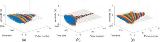
(Color online) The extracted call pulses. (a) 17 pulses from the first dataset. (b) 40 pulses from the second dataset. (c) 26 pulses from the third dataset.

FIG. 3.

(Color online) The extracted call pulses. (a) 17 pulses from the first dataset. (b) 40 pulses from the second dataset. (c) 26 pulses from the third dataset.

Close modal

For a better display effect, a zeros-padding operation is performed at both ends of the pulses, but this is not the case when they are calculated. The sample size of the bat pulses varies greatly, with the maximum being close to 1000 and the minimum being less than 100. The pulses in the first two phases usually contain two harmonics, and the three-harmonic pulses are used at the capturing phase, so only the first and second harmonics are considered for estimation in Sec. V B.

B. Validation

In this section, we first verify the feasibility of the parameter estimation flow in Table I with a bat pulse, and then apply the processing to all pulses along with a comparison with the estimation using FRFT. Setting the delay range to 0∼3 times the duration of the pulse and a step of a sampling period, the waveform of the 10th pulse from the second dataset and its HST are shown in Fig. 4. A 2D spectral peak with a delay of 0.69 ms and a scale of –81.9 is found in the HST image. According to Eq. (27), the starting frequency and chirp rate of the first harmonic are estimated as 119.22 kHz and 0.0122, respectively. To estimate the parameters of the second harmonic, a red-marked window is set to filter out the first harmonic, and using Eq. (29), the filtered signal is obtained, as shown in Fig. 5.

FIG. 4.

(Color online) Parameter estimation of the first harmonic. (a) Waveform of the bat call pulse. (b) HST of the pulse.

FIG. 4.

(Color online) Parameter estimation of the first harmonic. (a) Waveform of the bat call pulse. (b) HST of the pulse.

Close modal

FIG. 5.

(Color online) Performing scaling filtering. (a) Scaling filter. (b) The filtered signal.

FIG. 5.

(Color online) Performing scaling filtering. (a) Scaling filter. (b) The filtered signal.

Close modal

Finally, the HST of the filtered signal is calculated as shown in Fig. 6(a). There is also a peak in the HST image, but it is significantly broadened in the delay dimension. According to the peak position, the starting frequency and chirp rate of the second harmonic are estimated as 210.61 kHz and 0.0054, respectively. As shown in Fig. 6(b), we plot the estimated instantaneous frequencies (IFs) calculated by Eq. (3) on the high-resolution TFD obtained by performing reassignment on the short-time Fourier transform of the signal.³⁸ It can be seen that the estimated IF curves indeed coincide with the real IFs. There are two issues worth noting. First, the harmonic energy of the bat call pulse varies greatly, and we cannot estimate the parameters of all harmonics by calculating HST only once, implying that scale filtering in Table I is necessary. In addition, there is a delay of 0.6 ms for the second harmonic in the pulse, resulting in the estimated starting frequency of 210.61 kHz being unreliable, but the chirp rate can be accurately estimated, consistent with the analysis in Sec. III A. Theoretically, we can roughly estimate the delay of the second harmonic by looking at the TFD of the pulse, but this workload is very large for many pulses, so the estimation of the starting frequency of the second harmonic will not be considered below.

FIG. 6.

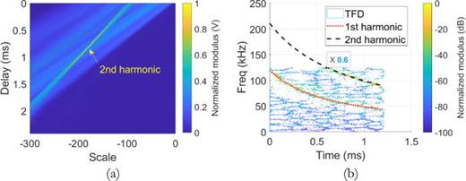
(Color online) Parameter estimation of second harmonic (a) HST of the filtered signal. (b) Estimated instantaneous frequencies of the two harmonics.

FIG. 6.

(Color online) Parameter estimation of second harmonic (a) HST of the filtered signal. (b) Estimated instantaneous frequencies of the two harmonics.

Close modal

Based on the processing above, the parameters of the 83 pulses are estimated. According to the parameter curves of the first harmonic in Fig. 7, it can be seen that the bats are always increasing the chirp rate of the first harmonic when searching, approaching, and capturing the prey, but the starting frequency is not adjusted in this way. In general, a high starting frequency is used in the middle phase, while a low starting frequency is adopted in the other two phases. An interesting phenomenon is that the parameter curves of the second dataset are closer to those of the third dataset, indicating that the HST may be useful in bat species identification, because the last two datasets are from the same species. However, such identification may not be achieved by analyzing only a pulse, but needing the analysis of multiple pulses and then performing a comparison of the parameter curves.

FIG. 7.

(Color online) Parameter estimation of first harmonic of the HFM-modeled bat call pulses using the proposed method. (a) Peak delay. (b) Peak scale. (c) Starting frequency. (d) Chirp rate.

FIG. 7.

(Color online) Parameter estimation of first harmonic of the HFM-modeled bat call pulses using the proposed method. (a) Peak delay. (b) Peak scale. (c) Starting frequency. (d) Chirp rate.

Close modal

The second harmonic has a known delay in the extracted pulses, resulting in the estimated starting frequency being unreliable according to the property of time-shift covariance of HST, although not erroneous, so only the chirp rate is estimated in Fig. 8. The trend is the same as that of the first harmonic, but the values are smaller. In addition, there are significant jumps in the estimated curves, indicating that the estimation is not good. There are two reasons to explain it: one is that the energy of the second harmonic is too weak and the sample size is smaller, and the second is that the signal-to-noise ratio of the filtered signal is low. In general, the estimation of the first harmonic is reliable for analysis, while that of the second harmonic is inclined to be used as a reference.

FIG. 8.

(Color online) Parameter estimation of second harmonic of the HFM-modeled bat call pulses using the proposed method. (a) Peak scale. (b) Chirp rate.

FIG. 8.

(Color online) Parameter estimation of second harmonic of the HFM-modeled bat call pulses using the proposed method. (a) Peak scale. (b) Chirp rate.

Close modal

To demonstrate the advantages of the proposed HST, a parameter estimation comparison with FRFT is necessary. Here, only the parameters of the first harmonics, i.e., the strongest harmonic, are taken into account. Setting the FRFT orders from 0 to 2, the starting frequency and the linear chirp rate of the first harmonic in the 83 pulses are estimated and shown in Fig. 9. In general, the estimation of the starting frequency is similar to that in Fig. 7(c), and the trend of the modulus of the linear chirp rate is also the same as that in Fig. 7(d), which is consistent with Eq. (7).

FIG. 9.

(Color online) Parameter estimation of the first harmonic of the bat call pulses using FRTF. (a) Starting frequency. (b) Linear chirp rate.

FIG. 9.

(Color online) Parameter estimation of the first harmonic of the bat call pulses using FRTF. (a) Starting frequency. (b) Linear chirp rate.

Close modal

However, the estimated starting frequency of the fifth through eighth pulses in Fig. 9(a) is anomalous, because they exceed 0.5 times sampling frequency, i.e., 125 kHz. To find the cause of the problem, we select the eighth and ninth pulses as processing objects, use FRFT and HST to estimate the parameters of the first harmonic, respectively, and then plot the estimated IFs to their TFD, as shown in Figs. 10 and 11. For the eighth pulse, the harmonic corresponding to the FRFT maximum peak is not the first harmonic, but the second harmonic, meaning that the estimated starting frequency of the fifth through eighth pulse in Fig. 9(a) is that of the second harmonic. In other words, FRFT is more suitable for estimating the parameters of the bat calls containing only a harmonic. In contrast, the proposed HST does not have such a problem. In addition, the estimated parameter curves using HST appear to be smoother, especially the curves of the peak scale and peak delay in Figs. 7(a) and 7(b).

FIG. 10.

(Color online) The estimated IFs obtained by FRFT. (a) Eighth bat call. (b) Ninth bat call.

FIG. 10.

(Color online) The estimated IFs obtained by FRFT. (a) Eighth bat call. (b) Ninth bat call.

Close modal

FIG. 11.

(Color online) The estimated IFS obtained by HST. (a) Eighth bat call. (b) Ninth bat call.

FIG. 11.

(Color online) The estimated IFS obtained by HST. (a) Eighth bat call. (b) Ninth bat call.

Close modal

C. Discussion

In this section, we try to explain the waveform strategy using the wideband ambiguity function. The wideband ambiguity function (WAF) of the waveform $s(t)$ is defined in the frequency domain as

${\text{WAF}}_S\left(\alpha ,\tau \right)={\int }_{-\infty }^{\infty }S\left(f\right)\frac{1}{\sqrt{\alpha }}{S}^{\ast }\left(\frac{f}{\alpha }\right){\mathrm{e}}^{\mathrm{i}2\pi f\tau }\mathrm{d}f,$

(39)

where $S(f)$ is the spectrum of $s(t)$⁠, $\alpha$ is the Doppler compression factor, $\alpha =(\mathrm{c}+v)/(\mathrm{c}-v)$⁠, $\mathrm{c}$ is the speed of sound, and $v$ is the relative velocity between the bat and its prey. Substituting Eq. (8) into Eq. (39) yields the wideband ambiguity function of the $n$th harmonic as

${\text{WAF}}_{S_n}\left(\alpha ,\tau \right)={\mathrm{e}}^{-\mathrm{i}2\pi (1/k_n)\text{ln}\hspace{0.17em}\left(\alpha \right)}\frac{1}{\sqrt{\alpha }{k}_n}{\int }_{f_{1,n}}^{f_{2,n}}\frac{1}{f^2}{\mathrm{e}}^{\mathrm{i}2\pi \alpha -1/\alpha 1/k_n{f}_{1,n}f}\mathrm{d}f,$

(40)

with the maximum value at

it can be seen that there is an unavoidable ranging bias, which is proportional to the IPD.³⁹ Since the Doppler compression factor is related to the sound speed and the relative velocity between the bat and prey, the adoption of decreasing IPD will be beneficial to reduce the ranging bias, as shown in Fig. 12. As to the first and 17th pulse in first dataset, when the factor is 1.2, i.e., the relative velocity between the bat and its prey is about 30 m/s with the speed of sound of 340 m/s, the bias of the first pulse observed from the WAF plot is about 0.22 ms, while that of the 17th pulse is only 0.04 ms. Because the parameters of the bat call pulse are set depending on the particular task to be carried out, it is easier to capture the target using the waveforms with higher-ranging accuracy if the target has already been judged to be the prey. The conclusion above has been made for a long time,¹² but not been supported by the estimated parameters so far, meaning that the results in this paper are significant. It must be admitted that the bats may not employ correlation detection used in the synthetic systems of radar and sonar, but a complex technique or model;⁴⁰ however, the analysis above is still meaningful for the improvement of the biomimetic technologies.

FIG. 12.

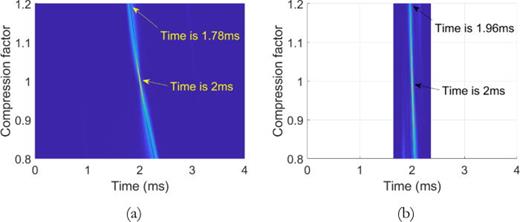
(Color online) Wideband ambiguity function. (a) First pulse. (b) 17th pulse.

FIG. 12.

(Color online) Wideband ambiguity function. (a) First pulse. (b) 17th pulse.

Close modal

VI. CONCLUSION

To estimate the parameters of the HFM-modeled bat calls, this paper proposes a transform, namely HST. HST is a linear and reversible transform with the properties of time-shift covariance, time-scaling covariance, and so on, very suitable for harmonic separation and parameter estimation of the HFM-modeled bat calls. The performance of HST is verified by three bat call datasets, and the estimated parameters show that bats are always increasing the chirp rate of the harmonics when searching, approaching, and capturing the prey, meaning that bats are very concerned about the ranging accuracy of the waveforms, which is consistent with the radar—sonar–related theory. In addition, the high starting frequency is often used in the approaching phase, while the low starting frequency is adopted in the other two phases. It should be noted that the IPD of the HFM-modeled bat calls is larger in the first phases, requiring a large delay range when HST is calculated. To reduce the computational amount, an idea is to take a large step for coarse search, and then take a small step for fine search. Future research is to apply HST to analyze the HFM-like calls of other mammals,⁴¹ as well as to the areas involving HFM signal processing.

ACKNOWLEDGMENTS

This work was supported by the National Natural Science Foundation of China (Grant Nos. 62101593, 62271498, and 62101583).

AUTHOR DECLARATIONS

Conflict of Interest

The authors have no conflicts to disclose.

DATA AVAILABILITY

APPENDIX A

The expression of the $n$th HFM component is

$s_{n}t=e^{i2\pi (1/k_n)\mathit{\text{ln}}1+k_n{f}_{1,n}t},$(A1)

assuming that the duration of $s_n(t)$ is infinite. According to the principle of stationary phase, first taking the integral phase term of the Fourier transform of $s_n(t)$ yields

$\varphi \left(t,f\right)=2\pi \hspace{0.17em}\text{ln}\hspace{0.17em}\left(1+k_n{f}_{1,n}t\right)/k_n-2\pi ft,$(A2)

its derivatives are given by

${\varphi }^{\prime }\left(t,f\right)=2\pi /\left[t+1/\left(k_n{f}_{1,n}\right)\right]k_n-2\pi f,$(A3)

${\varphi }^{″}\left(t,f\right)=-2\pi /{\left[t+1/\left(k_n{f}_{1,n}\right)\right]}^2{k}_n.$(A4)

Setting ${\varphi }^{\prime }(t,f)=0$⁠, the stationary point $t_0$ is obtained as

Finally, the spectrum of $s_n(t)$ is derived as

$S_n\left(f\right)\approx \left({\mathrm{e}}^{\mathrm{i}\frac{3}{4}\pi }{\mathrm{e}}^{-\mathrm{i}2\pi (1/k_n)}\frac{1}{2\sqrt{k_n}}\right)\frac{1}{f}{\mathrm{e}}^{\mathrm{i}2\pi (1/k_n{f}_{1,n})f}{\mathrm{e}}^{\mathrm{i}2\pi (1/k_n)\text{ln}\hspace{0.17em}\left(f_{1,n}/f\right)},\hspace{1em}f>0,$(A6)

where the first part is a complex constant, the second part implies that the spectrum envelope is inversely proportional to frequency $f$⁠, and the third part is a product of two complex exponents.

APPENDIX B

The kernel functions of the HST are

${\Upsilon }_{\tau }\left(c,f\right)=\frac{1}{\sqrt{f}}{\mathrm{e}}^{-\mathrm{i}2\pi f\tau }{\mathrm{e}}^{-\mathrm{i}2\pi c\hspace{0.17em}\text{ln}\hspace{0.17em}f},$(B1)

where $\tau$ is delay, $c$ is scale, and $f$ is frequency. The orthogonality of the HST can be obtained according to the double integrals below:

$\begin{array}{c}{\int }_{-\infty }^{\infty }{\int }_0^{\infty }{\gamma }_{\tau }^{\ast }\left(c^{\prime },f\right){\gamma }_{\tau }\left(c,f\right)\mathrm{d}f\mathrm{d}\tau ={\int }_{-\infty }^{\infty }{\int }_0^{\infty }\frac{1}{\sqrt{f}}{\mathrm{e}}^{\mathrm{i}2\pi f\tau }{\mathrm{e}}^{\mathrm{i}2\pi c^{\prime }\hspace{0.17em}\text{ln}\hspace{0.17em}f}\frac{1}{\sqrt{f}}{\mathrm{e}}^{-\mathrm{i}2\pi f\tau }{\mathrm{e}}^{-\mathrm{i}2\pi c\hspace{0.17em}\text{ln}\hspace{0.17em}f}\mathrm{d}f\mathrm{d}\tau ={\int }_{-\infty }^{\infty }\mathrm{d}\tau {\int }_0^{\infty }{\mathrm{e}}^{\mathrm{i}2\pi \left(c^{\prime }-c\right)\hspace{0.17em}\text{ln}\hspace{0.17em}f}\mathrm{d}\left(\text{ln}\hspace{0.17em}f\right)=\delta \left(c^{\prime }-c\right),\end{array}$(B2)

$\begin{array}{c}{\int }_{-\infty }^{\infty }{\int }_{-\infty }^{\infty }{\gamma }_{\tau }^{\ast }\left(c,f^{\prime }\right){\gamma }_{\tau }\left(c,f\right)\mathrm{d}c\mathrm{d}\tau ={\int }_{-\infty }^{\infty }{\int }_{-\infty }^{\infty }\frac{1}{\sqrt{f^{\prime }}}{\mathrm{e}}^{\mathrm{i}2\pi f^{\prime }\tau }{\mathrm{e}}^{\mathrm{i}2\pi c\hspace{0.17em}\text{ln}\hspace{0.17em}{f}^{\prime }}\frac{1}{\sqrt{f}}{\mathrm{e}}^{-\mathrm{i}2\pi f\tau }{\mathrm{e}}^{-\mathrm{i}2\pi c\hspace{0.17em}\text{ln}\hspace{0.17em}f}\mathrm{d}c\mathrm{d}\tau ={\int }_{-\infty }^{\infty }{\mathrm{e}}^{\mathrm{i}2\pi \left(f^{\prime }-f\right)\tau }\mathrm{d}\tau \frac{1}{\sqrt{f}\sqrt{f^{\prime }}}{\int }_{-\infty }^{\infty }{\mathrm{e}}^{\mathrm{i}2\pi \left(\text{ln}\hspace{0.17em}{f}^{\prime }-\text{ln}\hspace{0.17em}f\right)c}\mathrm{d}c=\delta \left(f^{\prime }-f\right),\end{array}$(B3)

$\begin{array}{c}{\int }_0^{\infty }{\int }_{-\infty }^{\infty }{\gamma }_{{\tau }^{\prime }}^{\ast }\left(c,f\right){\gamma }_{\tau }\left(c,f\right)\mathrm{d}c\mathrm{d}f={\int }_0^{\infty }{\int }_{-\infty }^{\infty }\frac{1}{\sqrt{f}}{\mathrm{e}}^{\mathrm{i}2\pi f{\tau }^{\prime }}{\mathrm{e}}^{\mathrm{i}2\pi c\hspace{0.17em}\text{ln}\hspace{0.17em}f}\frac{1}{\sqrt{f}}{\mathrm{e}}^{-\mathrm{i}2\pi f\tau }{\mathrm{e}}^{-\mathrm{i}2\pi c\hspace{0.17em}\text{ln}\hspace{0.17em}f}\mathrm{d}c\mathrm{d}f={\int }_{-\infty }^{\infty }\mathrm{d}c{\int }_0^{\infty }\frac{1}{f}{\mathrm{e}}^{\mathrm{i}2\pi \left({\tau }^{\prime }-\tau \right)f}\mathrm{d}f\ne \delta \left(\tau -{\tau }^{\prime }\right).\end{array}$(B4)

REFERENCES

1. M. Denny, “  The physics of bat echolocation: Signal processing techniques,”  Am. J. Phys. 72,  1465 – 1477 ( 2004 ).

2. K. Ghose and  C. F. Moss, “  The sonar beam pattern of a flying bat as it tracks tethered insects,”  J. Acoust. Soc. Am. 114,  1120 – 1131 ( 2003 ).

3. W. J. Lee,  B. Falk, and  C. Chiu, “  Tongue-driven sonar beam steering by a lingual-echolocating fruit bat,”  PLoS Biol. 15,  e2003148 ( 2017 ).

4. D. Schoeppler,  H. U. Schnitzler, and  A. Denzinger, “  Precise Doppler shift compensation in the hipposiderid bat, Hipposideros armiger,”  Sci. Rep. 8,  1 – 11 ( 2018 ).

5. M. E. Bates,  J. A. Simmons, and  T. V. Zorikov, “  Bats use echo harmonic structure to distinguish their targets from background clutter,”  Science 333,  627 – 630 ( 2011 ).

6. S. Uday and  J. A. Simmons, “  Echolocating bats perceive natural-size targets as a unitary class using micro-spectral ripples in echoes,”  Behav. Neurosci. 133,  297 – 304 ( 2019 ).

7. B. C. Leavell,  J. J. Rubin,  C. J. McClure,  K. A. Miner,  M. A. Branham, and  J. R. Barber, “  Fireflies thwart bat attack with multisensory warnings,”  Sci. Adv. 4,  eaat6601 ( 2018 ).

8. J. J. Rubin,  C. A. Hamilton,  J. W. McClure,  B. A. Chadwell,  A. Y. Kawahara, and  J. R. Barber, “  The evolution of anti-bat sensory illusions in moths,”  Sci. Adv. 4,  eaar7428 ( 2018 ).

9. E. C. Teeling,  M. Scally, and  D. J. Kao, “  Molecular evidence regarding the origin of echolocation and flight in bats,”  Nature 403,  188 – 192 ( 2000 ).

10. N. B. Simmons,  K. L. Seymour, and  J. Habersetzer, “  Primitive Early Eocene bat from Wyoming and the evolution of flight and echolocation,”  Nature 451,  818 – 821 ( 2008 ).

11. S. Haykin,  Y. B. Xue, and  P. Setoodeh, “  Cognitive radar: Step toward bridging the gap between neuroscience and engineering,”  Proc. IEEE 100,  3102 – 3130 ( 2012 ).

12. M. Vespe,  G. Jones, and  C. J. Baker, “  Lessons for radar: Waveform diversity in echolocating mammals,”  IEEE Signal Process. Mag. 26,  65 – 75 ( 2009 ).

13. S. D. Gordon and  H. M. Hofstede, “  The influence of bat echolocation call duration and timing on auditory encoding of predator distance in noctuoid moths,”  J. Exp. Biol. 221,  jeb171561 ( 2018 ).

14. M. Smotherman,  M. Knörnschild,  G. Smarsh, and  K. Bohn, “  The origins and diversity of bat songs,”  J. Comp. Physiol. A 202,  535 – 554 ( 2016 ).

15. Z. Fu,  N. Xu,  G. Zhang,  D. Zhou,  L. Liu,  J. Tang,  P. H.-S. Jen, and  Q. Chen, “  Evoked potential study of the inferior collicular response to constant frequency-frequency modulation (CF-FM) sounds in FM and CF-FM bats,”  J. Comp. Physiol. A 205,  239 – 252 ( 2019 ).

16. R. A. Altes and  E. L. Titlebaum, “  Bat signals as optimally Doppler tolerant waveforms,”  J. Acoust. Soc. Am. 48,  1014 – 1020 ( 1970 ).

17. J. J. Kroszczynski, “  Pulse compression by means of linear-period modulation,”  Proc. IEEE. 57,  1260 – 1266 ( 1969 ).

18. R. Brabant,  Y. Laurent,  U. Dolap,  S. Degraer, and  B. Poerink, “  Comparing the results of four widely used automated bat identification software programs to identify nine bat species in coastal Western Europe,”  Belg. J. Zool. 148,  119 – 128 ( 2018 ).

19. S. Haykin, “  Cognitive radar: A way of the future,”  IEEE Signal Process. Mag. 23,  30 – 40 ( 2006 ).

20. X. L. Sheng,  C. P. Dong, and  L. X. Guo, “  A bioinspired twin inverted multiscale matched filtering method for detecting an underwater moving target in a reverberant environment,”  Sensors 19,  5305 ( 2019 ).

21. I. Djurović and  A. Wojciechowski, “  Quasi-maximum likelihood-based estimator of the hyperbolic frequency modulated signals,”  Digit, Signal Process. 142,  104194 ( 2023 ).

22. I. Djurović, “  Random sample consensus algorithm for the hyperbolic frequency modulated signals parameters estimation,”  Signal Process. 218,  109390 ( 2024 ).

23. X. D. Jiang and  S. L. Wu, “  A novel parameter estimation for hyperbolic frequency modulated signals using group delay,”  Digit, Signal Process. 116,  103114 ( 2021 ).

24. S. Yao,  Y. Zhang,  Y. Xu,  Y. Gu,  Q. Wu, and  X. Liu, “  An improved parameter estimation of HFM signals based on IRLS linear fitting of extracted group delay,”  Signal Process. 217,  109347 ( 2024 ).

25. J. Dicecco,  J. E. Gaudette, and  J. A. Simmons, “  Multi-component separation and analysis of bat echolocation calls,”  J. Acoust. Soc. Am. 133,  538 – 546 ( 2013 ).

26. J. Marsal,  M. Rudnicki,  A. Jedel,  R. Salamon, and  I. Kochanska, “  Mutual clutter suppression techniques for FM sonars,”  Arch. Acoust. 41,  721 – 729 ( 2016 ).

27. C. Xue,  Y. M. Gu, and  Z. X. Gong, “  Direction of arrival estimation of wideband hyperbolic frequency modulation signals using parameterized time-frequency analysis,”  Acta Acust. 48,  27 – 40 ( 2023 ).

28. S. Parsons,  C. W. Thorpe, and  S. M. Dawson, “  Echolocation calls of the long-tailed bat: A quantitative analysis of types of calls,”  J. Mammal. 78,  964 – 976 ( 1997 ).

29. W. M. Masters and  S. C. Jacobs, “  The structure of echolocation sounds used by the big brown bat Eptesicus fuscus: Some consequences for echo processing,”  J. Acoust. Soc Am. 89,  1402 – 1413 ( 1991 ). 

30. D. A. Abraham,  Underwater Acoustic Signal Processing: Modeling, Detection, and Estimation, 1st ed. (  ASA Press,  Ellicott City, MD,  2019 ), pp.  48 – 51 . 

31. L. Cohen, “  The scale representation,”  IEEE Trans. Signal Process. 41,  3275 – 3292 ( 1993 ). 

32. Q. W. Xu,  H. F. Kuang,  L. Kneip, and  S. Schwertfeger, “  Rethinking the Fourier-Mellin transform: Multiple depths in the camera's view,”  Remote Sens. 13,  1 – 10 ( 2021 ). 

33. J. W. Yang,  Z. D. Lu,  Y. Y. Tang,  Z. Yuan, and  Y. J. Chen, “  Quasi Fourier-Mellin transform for affine invariant features,”  IEEE Trans. Image Process. 29,  4114 – 4129 ( 2020 ). 

34. A. O. Mac,  R. Gibb, and  K. E. Barlow, “  Bat detective-deep learning tools for bat acoustic signal detection,”  PLoS Comput. Biol. 14,  e1005995 ( 2018 ). 

35. A. De Sena and  D. Rocchesso, “  A fast Mellin and scale transform,”  EURASIP J. Adv. Signal Process. 2007,  1 – 9 . 

36. H. Sundaram,  S. D. Joshi, and  R. K. P. Bhatt, “  Scale periodicity and its sampling theorem,”  IEEE Trans. Signal Process. 45,  1862 – 1865 ( 1997 ). 

37. B. Ristic and  B. Boashash, “  Scale domain analysis of a bat sonar signal,” in  Proceedings of IEEE-SP International Symposium on Time-Frequency and Time-Scale Analysis, Philadelphia, PA ( 1994 ), pp.  373 – 376 . 

38. G. Yu, “  A multisynchrosqueezing-based high-resolution time-frequency analysis tool for the analysis of non-stationary signals,”  J. Sound Vib. 492,  115813 ( 2021 ). 

39. X. F. Song,  P. Willett, and  S. L. Zhou, “  Range bias modeling for hyperbolic-frequency modulated waveforms in target tracking,”  IEEE J. Ocean Eng. 37,  670 – 679 ( 2012 ). 

40. M. Park and  R. Allen, “  Pattern-matching analysis of fine echo delays by the spectrogram correlation and transformation receiver,”  J. Acoust. Soc Am. 128,  1490 – 1500 ( 2010 ). 

41. M. V. Reyes Reyes,  S. Baumann-Pickering,  A. Simonis,  M. L. Melcón,  J. Trickey,  J. Hildebrand, and  M. Iñíguez, “  High-frequency modulated signals recorded off the Antarctic peninsula area: Are killer whales emitting them?,”  Acoust. Aust. 45,  253 – 260 ( 2017 ). 

© 2024 Acoustical Society of America.   

 

PHS: A Pulse Sequence Method Based on Hyperbolic Frequency Modulation for Speed Measurement

Tao Ping

onlinelibrary.wiley.com

---

1. Introduction

The channel in the marine environment is a time-varying and space-varying channel [1]. The fading effect of the time-varying channel is divided into two situations:

• (1)  The frequency-domain fading effect caused by the frequency-varying characteristics of the channel, such as frequency dispersion and multipath
• (2)  Time-domain fading characteristics due to the time-varying characteristics of the channel, such as fluctuation and movement

In general, the so-called fading refers to the frequency-domain fading, and the time-domain fading generally refers to Doppler fluctuation. The unstable effect of pulse-truncated continuous wave (PCW) signal in the channel limits the effectiveness of speed measurement. Due to the Doppler invariant effect of HFM signal [2], in the underwater acoustic detection, the HFM signal is the most preferred [2–4]. However, some frequency bands have too much transmission loss in the channel, and a single HFM signal may not be able to detect the target.

In order to overcome the above limitations of speed measurement and ranging, a pulse sequence method based on HFM for speed measurement (PHS) is proposed, which uses HFM signals of different frequency bands and pulse widths in the sequence. Therefore, PHS method can not only measure the speed but also improve the accuracy of speed measurement and distance measurement. The main contributions of this paper are threefold:

• (1)  The PHS method employs HFM signals of different frequency bands and pulse widths in the sequence. And then, there are some problems under marine environments; for example, due to excessive propagation loss in certain frequency bands, the echo energy is insufficient and cannot effectively detect the target, which can be thus avoided
• (2)  Different combinations of HFM signals in the sequence can be coherent accumulation, and the signal-to-noise ratio (SNR) of the signals is improved. Therefore, the signals are more obvious
• (3)  The HFM signals in the sequence can mutually calculate the speed and distance of the target, reducing the calculation error caused by a single signal calculation, and the accuracy of velocity measurement and ranging is thus greatly improved

In Peng et al. [5], a joint linear frequency modulation and hyperbolic frequency modulation approach for speed measurement (JLHS) is proposed. The JLHS method uses the same pulse width and frequency band of positive and negative frequency modulation signals (LFM+HFM) for speed measurement and ranging. On the other hand, two signal modulation methods are required to be opposite in JLHS. Compared with JLHS, in the PHS method, the HFM signals are only not to be completely consistent, which relaxes the requirements of bandwidth and pulse width and makes it more suitable for general conditions. On the other hand, since the tolerance of LFM to moving targets is far less than that of HFM, when the target speed is too high, LFM will have no peak output after matched filtering, and thus, JLHS cannot realize ranging and speed measurement.

In our previous work [6], a speed measurement method of combined HFM signals (SCH) is proposed, which employs positive and negative HFM signals for speed measurement and ranging. It is well known that the channel in the marine environment is a time-varying and space-varying channel. Due to the filtering effect of the marine environment, the HFM signal of a single frequency band may cause excessive propagation loss, and the echo energy may be too weak to detect the target. Compared with SCH, in the PHS method, the HFM signals in pulse sequence adopt different frequency bands, and the more pulse forms in the pulse sequence, the easier it is for more echoes to return. Therefore, HFM pulse sequence signals are more conducive to engineering use.

2. Related Works

A new polyphase pulse compression code is proposed by Yang and Sarkar [7], which is derived from the stepwise approximation of the phase curve of a hyperbolic FM-chirp signal. And they solve the problem of relatively high sidelobe levels without Doppler effect by employing appropriate window functions. In multiuser communication systems (e.g., such as multiuser radar and sonar and multiple-access spread-spectrum communication systems), there has always been a problem, that is, the problem of frequency-hopping codes, which was successfully solved by Maric and Titlebaum [8]. The construction of a new family of frequency-hopping codes is given, and it is shown that hyperbolic frequency-hopping codes have almost ideal properties and can be used in two types of systems. To address the problem of conveniently handling the received energy while transmitting and receiving modulated energy, Whyland ([9]) proposed the use of Doppler-insensitive waveforms to modulate energy pulses or subpulses to probe a defined environment. For the sonar velocity measurement problem, many scholars are currently conducting research. Shao et al. [10] proposed the use of HFM+PCW-combined signal at the Western Acoustics Conference. The HFM signal is used for ranging, and the PCW is used for velocity measurement. The PCW signal cannot consistently and effectively contact the target due to its unstable operation in the sound field. Therefore, PCW can achieve speed measurement in echoes with high SNR. When the SNR does not meet the requirements slightly, PCW will cause a large speed measurement error. Peng et al. [5] used HFM and LFM signals with the same frequency band and the same pulse width for speed measurement. This method takes advantage of the advantages of HFM and LFM at the same time, but it needs to meet certain requirements for SNR. When the SNR is too low, LFM has no peak output, resulting in failure of distance and speed calculation. HFM waveform has inherent Doppler invariant characteristics. Based on this, Meng et al. [4] worked out the constraints on HFM parameters in order to better reduce the multiple-access interference at the transmission end. The multipath and scaled underwater channel effects are reduced due to additional limitations on the frequency modulation rate. After extensive experimental comparisons of the proposed signaling scheme with HFM-based CDMA schemes, the improved performance of the new scheme is demonstrated. In Gini and Giannakis [11], the parameter estimation problem of the combination of polynomial phase signal and HFM is well solved. In Xin [12], an improved preamble waveform UMD-HFM is proposed. On the basis of the UD-HFM signal, a blank interval is added to resist the delay expansion and Doppler delay of the multipath channel to avoid waveform stacking shown, but the use and variation of blanking intervals are not indicated. In order to overcome the multipath effect and the strong Doppler effect of the shallow sea, the HFM-SS spread-spectrum modulation is used for communication [13], and the Doppler invariance of HFM is fully utilized. However, this paper only considers a single HFM and does not consider using the relationship between the HFMs in spread-spectrum modulation to solve the Doppler. During the communication process, UD-HFM uses the positive and negative HFM as the preamble signal to estimate the Doppler velocity [14]. In order to avoid waveform superposition, the mute time is increased. This method defaults to the invariance of the mute time in the process of calculating the Doppler factor, but the mute time is changed at this time. On the other hand, the UD-HFM signal in this paper requires that the two HFMs are signals of the same frequency band and the same pulse width, which is a waste of frequency band utilization. At the same time, it is not conducive to overcoming the frequency selection characteristics of ocean channels. Liu et al. [15] presented mathematical formulations for multipath propagation model and the corrupted echoes. The impact of the multipath propagation on target detection is then analyzed. In addition, in order to remove the ghost targets, a simple but effective algorithm is proposed. Numerical simulation results show the satisfactory performance. In Murray [16], an extended matching filter is introduced into the HFM waveform in active sonar systems and provides an accurate closed-form solution to Doppler bias in arrival time estimates. The solution is suitable for broadband and narrowband HFM signals.

3. Ranging and Speed Measurement Based on PHS Method

According to the properties of the Fourier transform, the convolution of two signals in the time domain is equivalent to the multiplication of their FFT in the frequency domain. Convolution in the time domain can also realize the velocity measurement function. However, the convolution calculation in the time domain is more complex. This is because the convolution calculation in the time domain requires the signal to multiply and add different shift points, which requires a large amount of computation and more hardware memory, while the FFT multiplication in the frequency domain is simple to calculate and easier to implement. Therefore, in this paper, we use HFM signals of different frequency bands and pulse widths in the sequence to realize speed measurement.

Figure 1 shows the working process of the PHS method. When active sonar works, the transmitting system transmits several acoustic signals with specific information into the seawater separately, such as HFM signal 1 and HFM signal 2, which are called the transmitting signals. When the transmitting signals travel in seawater and meet targets, the echo signals will be generated. The echo signals propagate in the sea water according to the law of propagation and reach the hydrophone, which convert the acoustic signals into electrical signals. The electrical signals are processed by the signals (matching filtering and obtaining the peak time of each HFM signal, designing the function model and calculating, and coherent integration MTD operating between pulse trains) to obtain the distance and speed of the target.

The work processing of the PHS method.

4. The Principle of Velocity Measurement by Pulse Sequence Signals

Let T denote the pulse width of the HFM signal, f₀ denote the starting frequency of the HFM signal, f₁ denote the ending frequency of the HFM signal, and s_s(t) denote the HFM transmitting signal changing over time. Then, s_s(t) can be calculated by

(1)

where t^′ = (T/2) × ((f₁ + f₀)/(f₁ − f₀)) and k = (Tf₀f₁)/(f₁ − f₀).

Let f_s(t) denote the instantaneous frequency of HFM transmitting signal, and it can be expressed as the derivative of the signal phase with respect to time divided by 2π. We have [6]

(2)

The velocity of the target is denoted by v. When the target is moving at a speed of v, the relative motion between the sonar and the target results in a pulse width of T for the transmitted signal. At the receiving point, the transmitted signal becomes a signal with pulse width of T/η. Therefore, the pulse width of the echo is linearly compressed or stretched η times. And we have [6]

(3)

where c represents the speed of sound in water and c = 1500 m/s.

Let s_r(t) represent the received echo signal. Due to the radial movement between the target and the sonar platform, s_r(t) can be calculated as

(4)

Let f_r(t) represent the instantaneous frequency of the received echo. According to Equation (4), f_r(t) can be expressed as

(5)

Since the HFM signal is insensitive to Doppler, the HFM signal has the characteristic of Doppler invariance [2]. Moreover, the change rule of the instantaneous frequency of the received signal remains unchanged, except that the instantaneous frequency f_s(t) of the original signal is shifted by a time t₀, where t₀ represents matched filter delay caused by target Doppler. We have [6]

(6)

Based on Equation (2), Equation (5), and Equation (6), t₀ can be computed as

(7)

In practical applications, the arrival time of the target is unknown, and the Doppler-induced delay t₀ and the uncertainty of the arrival time of the target coexist, resulting in a single HFM signal unable to obtain a resolvable Doppler-induced delay t₀, as shown in Figure 2.

The delay after matched filtering caused by velocity.

Frequency band and pulse width are the two key elements to consider when HFM signals are used for object detection. In order to obtain the delay difference and delay ratio after matched filtering, two HFM pulse signals (HFM pulse signal 1 and HFM pulse signal 2) in the pulse sequence are adopted.

Note: in this paper, HFM signal represents HFM pulse signal.

HFM signal 1: the starting frequency is denoted by f₁₀, the ending frequency is denoted by f₁₁, and the pulse width is denoted by T₁.

HFM signal 2: the starting frequency is denoted by f₂₀, the ending frequency is denoted by f₂₁, and the pulse width is denoted by T₂.

For a moving target, the time delay t_d1 of HFM signal 1 can be computed as Equation (8). On the other hand, the time delay t_d2 of HFM signal 2 can be computed as Equation (9).

(8)

(9)

where

(10)

Dividing Equation (8) by Equation (9), we can obtain the ratio as follows:

(11)

Now, let us derive the formulas of both ranging and speed measurement. Assume that the velocity v of the target towards the sonar system is positive. Two combined HFM signals in pulse sequence, HFM signal 1 and HFM signal 2, are transmitted. Let t₁ and t₂ represent the time of maximum matched filter of HFM signal 1 and the time of maximum matched filter of HFM signal 2, respectively. We have

(12)

(13)

According to the above two equations (Equations (12) and (13)), the distance R between the sonar and the target can be computed as

(14)

Another form of R is

(15)

where arrival time of the pulse is denoted by τ.

According to Equations (14) and (15), τ is obtained.

(16)

And then, based on Equation (12) and Equation (16), t_d1 can be computed by

(17)

According to Equations (3), (16), and (17), the target speed v can be obtained.

(18)

where

(19)

The ideal transmission channel is an infinite space composed of lossless and uniform medium, and during the propagation process, the signal cannot have any distortion. However, it is well known that the seawater medium space is a lossy heterogeneous medium space. In addition to general absorption and diffusion, the signal in sea water is also affected by multipath effect, channel time-varying and fluctuation effect, which result in the broadening of the echo and the difficulty in distinguishing the echo position of the combined echo signal. In order to achieve accurate speed measurement, we employ multiple HFM signals in pulse sequence, and the HFM signals adopt different frequency bands, and the more pulse forms in the pulse sequence, the easier it is for more echoes to return. Therefore, the signals are more obvious. Based on the above analysis, we can see that the HFM pulse sequence signals are more conducive to engineering use.

5. Moving Target Detection (MTD) between Pulse Sequences

The moving target detection (MTD) processing in pulse sequence is shown in Figure 3. It is assumed that the number of peak output of different HFM signals in the pulse sequence is N. Using the N peak outputs of pulse sequence to perform calculation in pairs, the speed and the corresponding distance can be obtained. Therefore, the total number of speeds and corresponding distances of the target is . However, since the ocean environment changes in time and space, the ocean channel is equivalent to a filter. The signal in some frequency bands has too much propagation loss, resulting in too low signal energy in the echo that cannot be effectively detected. On the other hand, although some echoes can be detected, the SNR is too low, and the noise leads to an error between the arrival time of the signal and the actual arrival time of the echo of the target. Therefore, the peak outputs with high SNR are selected in the pulse sequence to calculate the speed and distance, which will make the calculation results more accurate.

Signal processing diagram of pulse sequences.

6. Processing between Pulse Sequences

6.1. Incoherent Integration

Modelling the received echo sequence, that is, removing the phase information, for cross-period addition is called noncoherent integration or integration after detection. Generally speaking, since noncoherent integration does not utilize phase information, its detection performance is inferior to that of coherent integration. The difference between coherent integration and noncoherent integration is called detection loss. The detection loss is related to the SNR of the input. The larger the SNR is, the smaller the detection loss is. To take an extreme example, when the SNR is infinite (i.e., the noise is zero), the result of noncoherent integration is the same as that of coherent integration, and then, the detection loss is zero. In fact, as long as the input SNR is greater than 1, the detection loss is relatively small, and then, the coherent integration can be replaced by noncoherent integration. On the one hand, noncoherent integration is relatively simple to implement in engineering, and there is no strict coherence requirement for the system. On the other hand, for most moving targets, the fluctuation of the echo signals will obviously destroy the phase coherence of the adjacent echo signals. Therefore, even if the radar system has good coherence, it is difficult to obtain ideal coherent integration for undulating echoes. Therefore, although the SNR of noncoherent integration is not as good as coherent integration, noncoherent integration is often used in many cases [17]. However, noncoherent integration does not make full use of the phase of the signal, and then, the gain ratio is smaller than that of coherent integration.

6.2. Coherent Integration

Using the velocity and the corresponding distance, the echo signals are transplanted to the same starting point to carry out coherent integration MTD operation. And the coherent integration MTD is an integration method to improve the SNR of the target, which is generally performed on the complex envelope of the intermediate frequency signal or the zero intermediate frequency signal. Moreover, the coherent integration MTD retains the phase relationship between the received pulses and can increase the accumulated signal energy. That is, coherent integration utilizes the phase information of all the pulses. It is assumed that the total number of pulse echoes received during a pulse accumulation period is N, and each pulse cycle is divided into M distance gates. Discrete sampling is carried out for N pulse echoes, respectively, and let x_nm represent the sampling data on the mth distance gate of the nth pulse echo. Then, the sampling data of N pulse echo sequences can be expressed as a data of N∗M dimension, as shown in Figure 4. The signal amplitude can be greatly increased by the following: (1) M distance gates are fast time steps, and pulse compression processing is carried out. (2) N pulse echoes are slow time steps, and coherent pulse integration MTD is performed. The distance and velocity obtained in Section 4 are used to remove the signal delay in the pulse sequences, which is caused by the Doppler movement of the target. After the echo signals are rearranged, MTD operation is carried out, and then, a signal gain of N times can be achieved.

Diagram of coherent integration.

The time complexity of the proposed PHS method will be given by the following analysis. It is assumed that the number of the HFM signals in the pulse sequences is N. Since echo signal in each pulse sequence needs to be matched and filtered separately, the time complexity is O(N). On the other hand, during space beamforming, due to different frequency bands in the sequences, separate beamforming is required, so the space complexity is O(N). When the signal frequency bands in the sequences are the same and the pulse widths are different, the beamforming can only be done once, and the spatial complexity is thus O(1).

7. Simulation and Results

7.1. Simulation Settings

Three simulated environments were used for the performance analysis. In the following simulated environments, the distance between the sound source and the target is 7.5 km, the speed of the target is 14 m/s, the SNR = −10 dB, and the sample frequency f_sa = 7000 Hz. Here, the frequency band is denoted by F_s, and the pulse width is denoted by T_s.

Simulated environment 1: the HFM pulse sequences consist of the following HFM signals: for HFM signal 1, F_s is 200 Hz-1000 Hz, and the pulse width is 1 s. For HFM signal 2, F_s is 300 Hz-1200 Hz, and T_s is 2 s. For HFM signal 3, F_s is 400 Hz-1400 Hz, and T_s is 3 s. For HFM signal 4, F_s is 500 Hz-1600 Hz, and T_s is 4 s. For HFM signal 5, F_s is 600 Hz-1900 Hz, and T_s is 6 s.

Simulated environment 2: the HFM pulse sequences consist of the following HFM signals: for HFM signal 1, F_s is 100 Hz-200 Hz, and T_s is 1 s. For HFM signal 2, F_s is 700 Hz-900 Hz, and T_s is 2 s. For HFM signal 3, F_s is 1000 Hz-1200 Hz, and T_s is 3 s. For HFM signal 4, F_s is 1700 Hz-1900 Hz, and T_s is 4 s.

Simulated environment 3: the HFM pulse sequences consist of the following HFM signals: for HFM signal 1, F_s is 100 Hz-200 Hz, and T_s is 2 s. For HFM signal 2, F_s is 1000 Hz-700 Hz, and T_s is 3 s. For HFM signal 3, F_s is 1000 Hz-1300 Hz, and T_s is 3 s. For HFM signal 4, F_s is 1100 Hz-1300 Hz, and T_s is 1 s.

7.2. Simulation Results

For simulated environment 1, the performance analysis is shown in Figures 5 and 6. The numerical results of PHS are given in Table 1. From Figure 5, it can be seen that, after matched filtering, the signal echo time of HFM signal 1, HFM signal 2,HFM signal 3, HFM signal 4, and HFM signal 5 is 10.0236 s, 10.0502 s, 10.0792 s, 10.1096 s, and 10.1652 s, respectively. Figure 6 shows the MTD operation based on pulse sequence method. According to Equation (18), the value of v is 13.9914 m/s. It can be seen from Table 1 that the speed measurement error and the ranging error of PHS are 0.061429% and 0%, respectively. The ranging error of HFM signal 1, HFM signal 2, HFM signal 3, HFM signal 4, and HFM signal 5 is 0.0236%, 0.502%, 0.792%, 1.096%, and 1.652%, respectively. Compared with HFM signal 1, HFM signal 2, HFM signal 3, HFM signal 4, and HFM signal 5, the ranging measurement accuracy of PHS is all improved by 100%.

Single HFM signal detection under simulation environment 1.

Pulse sequence method based on HFM signal under simulation environment 1.

Table 1. For simulated environment 1: comparison of simulation results.

Echo time of single signal (s)					Ranging of single signal (km)					Ranging of PHS (km)	Speed of PHS (m/s)
HFM signal 1	HFM signal 2	HFM signal 3	HFM signal 4	HFM signal 5	HFM signal 1	HFM signal 2	HFM signal 3	HFM signal 4	HFM signal 5
10.0236	10.0502	10.0792	10.1096	10.1652	7.5177	7.53765	7.5594	7.5822	7.6239	7.5	13.9914

Ranging error of PHS	Speed measurement error of PHS	Ranging error of single signal					Range accuracy improvement ratio compared to
		HFM signal 1	HFM signal 2	HFM signal 3	HFM signal 4	HFM signal 5	HFM signal 1	HFM signal 2	HFM signal 3	HFM signal 4	HFM signal 5
0%	0.061429%	0.236%	0.502%	0.792%	1.096%	1.652%	100%	100%	100%	100%	100%

For simulated environment 2, the performance analysis is shown in Figures 7 and 8. The numerical results of PHS are given in Table 2. From Figure 7, it can be seen that, after matched filtering, the signal echo time of HFM signal 1, HFM signal 2, HFM signal 3, and HFM signal 4 is 10.0376 s, 10.1696 s, 10.3392 s, and 10.7160 s, respectively. Figure 8 shows the pulse sequence method based on HFM signals. According to Equation (18), the value of v is 14.0019 m/s. It can be seen from Table 2 that the speed measurement error and the ranging error of PHS are 0.013571429% and 0%, respectively. The ranging error of HFM signal 1, HFM signal 2, HFM signal 3, and HFM signal 4 is 0.376%, 1.696%, 3.392%, and 7.16%, respectively. Compared with HFM signal 1, HFM signal 2, HFM signal 3, and HFM signal 4, the ranging measurement accuracy of PHS is all improved by 100%.

Single HFM signal detection under simulation environment 2.

Pulse sequence method based on HFM signal under simulation environment 2.

Table 2. For simulated environment 2: comparison of simulation results.

Echo time of single signal (s)				Ranging of single signal (km)				Ranging of PHS (km)	Speed of PHS (m/s)
HFM signal 1	HFM signal 2	HFM signal 3	HFM signal 4	HFM signal 1	HFM signal 2	HFM signal 3	HFM signal 4
10.0376	10.1696	10.3392	10.7160	7.5282	7.6272	7.7544	8.037	7.5	14.0019

Ranging error of PHS	Speed measurement error of PHS	Ranging error of single signal				Range accuracy improvement ratio compared to
		HFM signal 1	HFM signal 2	HFM signal 3	HFM signal 4	HFM signal 1	HFM signal 2	HFM signal 3	HFM signal 4
0%	0.013571429%	0.376%	1.696%	3.392%	7.16%	100%	100%	100%	100%

For simulated environment 3, the performance analysis is shown in Figures 9 and 10. The numerical results of PHS are given in Table 3. From Figure 9, it can be seen that, after matched filtering, the signal echo time of HFM signal 1, HFM signal 2,HFM signal 3, and HFM signal 4 is 10.0754 s, 9.8682 s, 10.245 s, and 10.1224 s, respectively. Figure 10 shows the pulse sequence method based on HFM signals. According to Equation (18), the value of v is 13.996 m/s. It can be seen from Table 3 that the speed measurement error and the ranging error of SPHS are 0.02857% and 0%, respectively. The ranging error of HFM signal 1, HFM signal 2, HFM signal 3, and HFM signal 4 is 0.754%, 1.318%, 2.45% and 1.224%, respectively. Compared with HFM signal 1, HFM signal 2, HFM signal 3, and HFM signal 4, the ranging measurement accuracy of PHS is all improved by 100%.

Single HFM signal detection under simulation environment 3.

Pulse sequence method based on HFM signal under simulation environment 3.

Table 3. For simulated environment 3: comparison of simulation results.

Echo time of single signal (s)				Ranging of single signal (km)				Ranging of PHS (km)	Speed of PHS (m/s)
HFM signal 1	HFM signal 2	HFM signal 3	HFM signal 4	HFM signal 1	HFM signal 2	HFM signal 3	HFM signal 4
10.0754	9.8682	10.245	10.1224	7.55655	7.40115	7.68375	7.5918	7.5	13.996

Ranging error of PHS	Speed measurement error of PHS	Ranging error of single signal				Range accuracy improvement ratio compared to
		HFM signal 1	HFM signal 2	HFM signal 3	HFM signal 4	HFM signal 1	HFM signal 2	HFM signal 3	HFM signal 4
0%	0.02857%	0.754%	1.318%	2.45%	1.224%	100%	100%	100%	100%

8. Conclusion

The fuzzy function of HFM signal has the shape of the blade, which makes the velocity and distance to be coupled together. Due to the Doppler frequency shift caused by the target movement, the peak value after the matched filtering has a time delay in the time domain, resulting in the failure of a single HFM to accurately range. In this paper, based on the time delay of signals with different frequency bands or different pulse widths, a pulse sequence method based on HFM for speed measurement (PHS) is proposed, which uses HFM signals of different frequency bands and pulse widths in the sequence. The proposed method can not only guarantee the speed measurement but also improve the accuracy of the speed measurement and distance measurement.

In future research, we will realize simulation in more complex scenarios, such as multitarget speed measurement and simulation in the presence of clutter.

Conflicts of Interest

The authors declare that they have no conflicts of interest.

Acknowledgments

This work was supported in part by the Shandong Smart Ocean Ranch Engineering Technology Collaborative Innovation Center, in part by the Shandong Agricultural Science and Technology Service Project (No. 2019FW037-4), in part by the research fund for high-level talents of Qingdao Agricultural University (No. 6631119041), and in part by the Shandong Technology Innovation Guidance Program (No. 2020LYXZ023).

A graphic showing the stiffness of Earth’s crust beneath Japan. The image reveals the boundary where Japan’s continental plate (large dark red patch) collides with the stiffer oceanic plate (dark blue patch). The smaller dark red patches in the center of the image are likely a magma system feeding Japan’s volcanoes (red triangles). The image was created using data collected with a new deformation imaging technique developed by researchers at UT Austin. Credit: Simone Puel 

 

New imaging technique uses Earth's warped surface to reveal rocky interior

phys.org

Science X

Summary

Researchers at the University of Texas at Austin developed a new computational technique called "deformation imaging" that allows scientists to look inside the Earth using surface mapping technology like GPS and INSAR. Here is a summary of the key points:

1. The method uses surface deformation data, primarily from GPS stations, but can also incorporate other geodetic data like InSAR (Interferometric Synthetic Aperture Radar).

2. The technique provides information about the rigidity of the Earth's crust and mantle, which is important for understanding earthquakes and geological processes.

3. The method was applied to GPS data from Japan's 2011 Tohoku earthquake to image the subsurface down to about 100 km.

4. It revealed the boundary between Japan's continental plate and the stiffer oceanic plate, as well as a possible deep magma reservoir feeding Japan's volcanoes.

5. The technique combines GPS data with computer modeling to create 3D images of the Earth's interior based on surface deformation.

6. It provides results comparable to seismic imaging but offers direct information about rock rigidity which could be used to predict its behavior.

7. The method could be applied to data from satellites like NASA's upcoming NISAR mission to study geologically hazardous regions.

8. It has the potential to be integrated with other geophysical techniques to provide a more comprehensive understanding of Earth's structure and dynamics.

9. The study demonstrates that lateral variations in elastic strength can be recovered using geodetic data alone if fault geometries are reasonably well known.

10. The approach opens up new possibilities for studying fault and volcano dynamics, especially when combined with InSAR deformation time series data. 

Researchers

The primary researchers involved in developing the deformation imaging technique, based on the information provided, are:

1. Simone Puel - Lead researcher, formerly at the University of Texas at Austin (UT Austin), now a postdoctoral scholar in Geophysics at the California Institute of Technology.

2. Thorsten W. Becker - Professor at the Jackson School of Geosciences, UT Austin.

3. Omar Ghattas - Professor at the UT Walker Department of Mechanical Engineering and UT Oden Institute for Computational Engineering and Sciences.

4. Umberto Villa - Research Scientist Optimization, Inversion, Machine Learning, and Uncertainty for Complex Systems.

5. Dunyu Liu - COMPUTATIONAL GEOSCIENTIST Associated with the Institute for Geophysics, Jackson School of Geosciences, UT Austin.

Puel et al. published the theory behind their method in Geophysical Journal International earlier in the same year. They also reference previous work by some of the same authors, such as Puel et al. (2022) and Hashima et al. (2016), which contributed to the development of this technique.

Deformation Imaging

Deformation imaging is a new computational technique developed by researchers at the University of Texas at Austin that allows scientists to look inside the Earth using surface mapping technology. Here's an overview of how it works:

1. Data collection: The method uses surface deformation data, primarily from GPS stations, but can also incorporate other geodetic data like InSAR (Interferometric Synthetic Aperture Radar).

2. Earthquake event: The technique relies on measuring surface deformations caused by large geological events, such as major earthquakes. In this case, they used data from Japan's 2011 Tohoku earthquake.

3. Computer modeling: The researchers construct a 3D computer model that treats the Earth as a simplified elastic material, allowing its elastic strength to vary in three dimensions.

4. Inverse problem solving: The method uses an "adjoint-based optimization" approach to invert the surface deformation data. This means it works backwards from the observed surface movements to infer the underlying structure.

5. Joint inversion: The technique can simultaneously solve for both the fault slip (earthquake movement) and the 3D variations in rock properties like rigidity (shear modulus).

6. Iterative process: The model repeatedly adjusts its parameters to find the best fit between predicted and observed surface deformations.

7. Resolution and depth: The resulting images can provide information about subsurface structures down to about 100 km depth, with the best resolution in areas with dense GPS coverage.

8. Output: The final output is a 3D map of variations in rock properties, particularly rigidity, which can reveal features like tectonic plate boundaries, zones of weakness, and potential magma reservoirs.

This method is innovative because it provides direct information about rock rigidity, which is crucial for understanding earthquake dynamics and geological processes. Unlike seismic imaging, which infers properties from wave velocities, deformation imaging uses the actual movement of the Earth's surface to determine the mechanical properties of the rocks below.

Artifacts

Artifacts of the research that could be used by other geologists include:

1. Open-source software: The researchers used open-source libraries  FEniCS and hIPPYlib for their computations. 

 

2. Computational framework: The adjoint-based optimization method they developed could be applied to other fault systems.

3. Mesh generation technique: They used the open-source software GMSH to generate 3D meshes for their finite element computations.

4. Data processing methods: Their techniques for handling and integrating various types of geodetic data (GPS, seafloor sensors, pressure gauges) could be valuable for other studies.

5. Inversion algorithms: The joint inversion method for simultaneously solving for fault slip and material properties could be adapted for other fault systems.

While the study focused on the Japan Trench and the 2011 Tohoku earthquake, the researchers suggest that their method could be applied to other geologically hazardous regions. They specifically mention that it could be used with data from NASA's upcoming NISAR satellite mission, which will map the entire globe.

Therefore, it seems likely that this technique could be applied to other tectonic boundaries like the San Andreas fault, since there is sufficient geodetic data available from extensive surveys. The researchers emphasize that their approach is especially promising for settings where densely sampled InSAR deformation time series are available, which could include many major fault systems around the world.

---

Surface mapping technology such as GPS, radar and laser scanning have long been used to measure features on the Earth's surface. Now, a new computational technique developed at The University of Texas at Austin is allowing scientists to use those technologies to look inside the planet.

The new technique, described by researchers as "deformation imaging," provides results comparable to seismic imaging but offers direct information about the rigidity of the planet's crust and mantle. This property is essential for understanding how earthquakes and other large-scale geological processes work, said Simone Puel, who developed the method for a research project at the University of Texas Institute for Geophysics while in graduate school at the UT Jackson School of Geosciences.

"Material properties like rigidity are critical to understand the different processes that occur in a subduction zone or in earthquake science in general," Puel said.

"When combined with other techniques like seismic, electromagnetic or gravity, it should be possible to actually produce a much more comprehensive mechanical model of an earthquake in a way that has never been done before."

Puel, who is now a postdoctoral scholar at the California Institute of Technology, published the theory behind his method in Geophysical Journal International earlier this year. A recent study published in June in Science Advances shows it in action. It used GPS data recorded during Japan's 2011 Tohoku earthquake to image the subsurface down to about 100 kilometers underground.

The image revealed the tectonic plates and volcanic system beneath the Japanese portion of the Pacific Ring of Fire, including an area of low rigidity that's thought to be a deep magma reservoir feeding the system—the first time such a reservoir has been detected using only surface information.

A GPS station atop the Sierra Nevada mountains. UT Austin researchers used GPS networks to image the planet’s interior. Credit: UNAVCO/NSF

The method relies on the fact that Earth's crust is a hodge-podge of rocky material with differing elastic properties. Some parts are more pliant, and other parts are more rigid. This causes the crust to contract and expand unevenly. During an earthquake, for example, the Earth vibrates in a way that reflects what it's made of, leaving the surface deformed in telltale ways.

To turn this uneven deformation into an image of the subsurface, the researchers constructed a computer model that treats the Earth as if it is a simplified elastic material, while allowing its elastic strength to vary in three dimensions.

The model then computed the subsurface rigidity based on how much the GPS sensors had moved in relation to one another during the earthquake. The result is a 3D picture of the Earth's interior based on changes on the surface.

An advantage of the new method is that it can use measurements made by satellites. These include NASA's upcoming NISAR spacecraft, a joint mission with the Indian Space Research Organization that will map the entire globe in very high resolution every 12 days.

Using the new technique, NISAR could offer important insights into some of the world's most geologically hazardous regions, said study co-author Thorsten Becker, a professor at the Jackson School. By continuously mapping the Earth's surface, the satellite will allow scientists to track structural changes in earthquake faults as they progress through their earthquake cycle.

Co-author Omar Ghattas, a professor at the UT Walker Department of Mechanical Engineering and UT Oden Institute for Computational Engineering and Sciences, said that the new method could be an important step to building digital twins of the Earth. These complex computer models perpetually improve themselves by identifying where to make new observations, then assimilating the new data.

More information: S Puel et al, An adjoint-based optimization method for jointly inverting heterogeneous material properties and fault slip from earthquake surface deformation data, Geophysical Journal International (2023). DOI: 10.1093/gji/ggad442

Simone Puel et al, Volcanic arc rigidity variations illuminated by coseismic deformation of the 2011 Tohoku-oki M9, Science Advances (2024). DOI: 10.1126/sciadv.adl4264

Citation: New imaging technique uses Earth's warped surface to reveal rocky interior (2024, July 2) retrieved 2 July 2024 from https://phys.org/news/2024-07-imaging-technique-earth-warped-surface.html

This document is subject to copyright. Apart from any fair dealing for the purpose of private study or research, no part may be reproduced without the written permission. The content is provided for information purposes only. 

Volcanic arc rigidity variations illuminated by coseismic deformation of the 2011 Tohoku-oki M9

Dunyu Liu

science.org

---

Abstract

Rock strength has long been linked to lithospheric deformation and seismicity. However, independent constraints on the related elastic heterogeneity are missing, yet could provide key information for solid Earth dynamics. Using coseismic Global Navigation Satellite Systems (GNSS) data for the 2011 M9 Tohoku-oki earthquake in Japan, we apply an inverse method to infer elastic structure and fault slip simultaneously. We find compliant material beneath the volcanic arc and in the mantle wedge within the partial melt generation zone inferred to lie above ~100 km slab depth. We also identify low-rigidity material closer to the trench matching seismicity patterns, likely associated with accretionary wedge structure. Along with traditional seismic and electromagnetic methods, our approach opens up avenues for multiphysics inversions. Those have the potential to advance earthquake and volcano science, and in particular once expanded to InSAR type constraints, may lead to a better understanding of transient lithospheric deformation across scales.

INTRODUCTION

Large-magnitude subduction zone earthquakes cause widespread deformation, including coseismic subsidence beneath volcanoes located hundreds of kilometers away from the rupture area (1, 2). Associated local deformation may indicate rheological heterogeneity associated with the magmatic plumbing system (3, 4) where the presence of high geothermal gradients (3, 5) and crustal intrusions (6, 7), for example, may mechanically weaken the rocks.

While geodetic observations have previously been used for inferences about elastic structure on global scales (8), here, we present the first direct inversion of coseismic crustal deformation for both upper mantle, margin-scale elastic properties and fault slip. We focus on northeastern Japan and invert coseismic surface displacements due to the 2011 Tohoku-oki M9 earthquake to investigate rigidity variations along the margin and specifically within the overriding plate’s volcanic arc. Low-seismic velocity beneath the volcanic arc in northeastern Japan have long been imaged by seismic tomography (9, 10), including for individual volcanoes such as Naruko (11, 12), and high v_P/v_s ratios at depth suggest the presence of fluids and/or partial melt (10, 13). The sources of these fluids may be attributed to dehydration metamorphic reactions of minerals from the subducting slab at ~100 km depth, above which many of the volcanic arcs worldwide are typically located (14, 15).

Beneath the volcanoes and inland northeastern Japan, the upper-plate structure exhibits shallow seismicity within the brittle deformation regime. In addition, deeper low-frequency earthquakes occur around active volcanoes, often associated with magmatic activity (9). In contrast, seismic activity is notably elevated and more widespread offshore, in particular along the primary thrust region beneath the landward slope of the Japan Trench. Several studies involving seismic, gravity, and residual topography analyses have linked the segmentation of megathrust events to material heterogeneities in the overriding plate (16, 17), suggesting a substantial influence of structural heterogeneities on earthquake nucleation and rupture style (18). For instance, Bassett et al. (16) proposed that variations in the forearc lithology of the upper plate played a key role in the along-strike variations in the 2011 Tohoku-oki M9 earthquake slip distribution. It is thus important to independently quantify the extent and distribution of the Earth’s rigidity structure within a fault and volcano dynamics context.

RESULTS

Joint inversion of geodetic data

We seek to infer variations in elastic parameters directly from coseismic geodetic deformation observations (19) associated with the 2011 Tohoku-oki M9. We use three-dimensional displacement information from 1283 permanent Global Positioning System (GPS) sensors, eight seafloor acoustic GPS sensors (GPS/A), and six pressure gauges (APG); the latter measure verticals only (20–22). The M9 resulted in major deformation (20–22), with ∼5-m displacements recorded horizontally in the eastern part of the Tohoku region on land, and over 30 m on the seafloor (Fig. 1A) with data corrected to remove aftershock effects (23, 24). Vertical deformation showed ∼5 m of uplift near the Japan Trench and ∼1 m of subsidence near the Pacific coast of Honshu. Observational errors for the inland and offshore stations are inferred to range from a few millimeters to several centimeters (table S1).

Fig. 1. Coseismic geodetic data, displacement residuals, and inferred fault slip distribution for homogeneous and heterogeneous structure.

(A) Coseismic deformation of the 2011 Tohoku-oki M9 earthquake (20–22). Yellow and white arrows indicate horizontal displacement vectors on different scales and uplift is represented by the background color. The red star is the Tohoku-oki epicenter, and the purple contour represents the 5-m slip contour from an earlier coseismic slip inversion (24). The dark red lines are major plate boundaries (61), and the red dashed line depicts the 100-km contour line of the subducting Pacific slab (62). (B and C) Displacement residuals (on different scale) and fault slip (5 m cyan contours) from our homogeneous medium slip inversion (B), and our joint inversion for fault slip and 3D shear modulus variations (C), as shown in Fig. 2. Mean values in averaging brackets indicate the root mean square (RMS) values (A) and residuals [(B) and (C)] of horizontal (u_h) and vertical (u_z) displacements, restricted to the map area on land.

We perform an inversion of the geodetic data; first for fault slip alone, and then for slip and three-dimensional (3D) rigidity variations (Materials and Methods). Our model domain covers a 3700 × 4600 km rectangular region around Honshu with a depth of 700 km. We refine the mesh around the epicenter and the central part of eastern Honshu (fig. S1), where we anticipate the highest information recovery from the geodetic data (Materials and Methods). Figure 1B shows the inferred fault slip and residuals between model predictions and horizontal and vertical coseismic deformation of our best homogeneous structure model. The misfit is at the ≈2 and ≈26% level for the horizontals and verticals on land, respectively (Fig. 1B). The horizontal and, more so, the vertical residuals are clearly not random but show spatially coherent patterns. Such residuals are also apparent in earlier homogeneous medium inversions (25). Their origin in terms of a contrast between strong slab and weak overriding plate and/or mantle has previously been explored by forward computations exploring the role of elastic heterogeneity (24–27).

Figure 1C shows that the residuals can be markedly reduced if we allow for 3D rigidity variations during a joint inversion for fault slip and rigidity, with the corresponding shear modulus variations shown in Figs. 2 and 3. In this case, root mean square (RMS) misfit values between model and geodetic data on land are roughly halved, to ≈1 and ≈16% for the horizontals and verticals, respectively (Fig. 1C and table S1). By jointly inverting for rigidity variations and coseismic slip, the remaining misfit patterns now lack any obvious, overall coherent structure. Only a small region in the eastern part of the Onikobe volcanic area shows overestimated vertical displacements.

Fig. 2. Map view of rigidity variations from the 3D joint inversion.

The shear modulus, or rigidity, variations (δμ) are shown relative to the background in percent for our preferred joint inversion (Fig. 1C) at depths of 5 km (A) and 75 km (B). Geodetic sites are marked with black circles, volcanoes (63) are denoted by orange triangles. Slip contours in 5-m intervals are represented with black contours. Plate boundaries, slab contours, and epicenter as in Fig. 1. Profiles indicated are shown in Fig. 3.

Open in viewer

Fig. 3. Vertical profiles illustrating rigidity (shear modulus) variations (δμ) obtained from the 3D joint inversion.

The corresponding profile locations are shown on Fig. 2. The orange line represents the topography and bathymetry, while the orange triangles indicate the locations of volcanoes (63). White and gray dots indicate the location of the GPS stations and the APG along the profiles, respectively. The black points correspond to seismicity with a M_w > 3.5 from the Japan Meteorological Agency Catalogue between 1973 and 2023. The black solid and dashed lines depict the geometry of the Pacific slab and the 100-km depth line, respectively. This depth region represents the level at which the release and upward migration of hydrous minerals’ metamorphic reactions within the subducting slab are considered to occur, contributing to the formation of the volcanic arc.

Open in viewer

The residual reduction is possible because deep elastic modulus variations have subtle but robust diagnostic surface deformation signatures for a given slip geometry (19, 27), and the data appear to resolve an overriding plate that is weaker than the slab and additional anomalies in the mantle wedge that are associated with the volcanic arc (Fig. 2). Comparing the slip distribution inferred assuming a homogeneous structure with the joint inversion (contours in Figs. 1, B and C, and colored figs. S2, A and B), we find similar slip distributions with most slip concentrated near the trench, consistent with previous inversions with prescribed 3D shear modulus variations (24, 26). The preferred joint inversion estimates a slightly lower maximum slip of 41 m compared to 46 m in the homogeneous case and has relatively smoother slip distribution, highlighting the trade-offs with fault-proximal structure. This reduction in slip magnitude broadly aligns with previous studies considering heterogeneous material structure in forward tests (24, 26, 27). Higher slip near the trench might be likely, e.g., from bathymetric surveys (28), within uncertainties (29, 30), for example, and additional constraints could be included in future slip inversions. In our tests, we also find a moderate trade-off of maximum slip with slab geometry (fault dip; figs. S2C and S8), whereas the 3D rigidity structure is quite stable with respect to fault dip (figs. S6 and S7).

Rigidity structure and weaker volcanic arc

Concentrations of more compliant material underneath the Japanese landmass correlate well with the location of volcanic centers between 37° and 42°N (Fig. 2) where GPS spatial coverage and resolution are high (fig. S3). On the basis of a number of synthetic tests, we found these features to be robust outcome of the inversion (e.g., figs. S4 and S5). At shallow depths (Fig. 2A), rigidity reductions of ∼15 to 25% are observed around Mt. Akitakoma (40°N), Mt. Kurikoma (39°N), Mt. Zao (38°N), and reductions between 25 and 35% are seen beneath Mt. Azuma (∼37.5°N) and Mt. Nasu (37°N). These volcanoes experienced notable subsidence during the 2011 Tohoku-oki event (1).

The presence of high geothermal gradients (3, 5), and presence of deep-seated hot plutonic bodies (6) in this area aligns with the rigidity reduction due to increased temperatures weakening the rocks. These weaker material anomalies are prominent within the uppermost 30 km, which corresponds to the average crustal thickness in northeastern Japan (31) and to the region of reported shallow seismicity (black dots in Fig. 3), some of which may be associated with the volcanic plumbing systems. Seismic tomography of the Japan arc (32, 33) suggests a correlation between the more compliant anomalies we image and low seismic velocity anomalies at shallow depths (Fig. 4).

Fig. 4. Comparison between rigidity and seismic velocity variations and density inference.

(A and B) Rigidity variations (δμ) from the 3D joint inversion (A; Fig. 3) and seismic velocity variations (33) (δv_s; B) of vertical C-D profile (Fig. 2). (C) Inference of density anomalies (δρ) calculated from rigidity variations and a smoothed version of the seismic tomographic model (B). Topographic elevation, slab geometry, volcano, and station locations as in Fig. 3.

An interesting observation in profile C-D of Fig. 3 is a lower rigidity region with a ~30% shear modulus reduction between 30 and 50 km depth beneath Naruko volcano, surrounded by a slightly stronger region (reduction below 20%). This deeper anomaly is well correlated with low-velocity anomalies and high v_P/v_s ratios observed beneath this volcano at these depths (11, 12, 34), possibly indicating the presence of a deeper magma reservoir. This deeper magma storage beneath Naruko, as well as shallower reservoirs beneath other volcanoes, may be directly connected to the source region of melt and fluids associated with metamorphic reactions within the subducting slab (35).

Notably, the volcanic low-rigidity anomalies in Figs. 2B and 3 align with the subducting slab interface reaching ~100 km depth, and the equivalent distance from the trench is typically associated with the main volcanic arc (14, 15). Shear modulus reductions between 8 and 12% are apparent at 75 km depth (Fig. 2) along the volcanic arc, suggesting the possible presence of fluids and/or melt at these depths. Mechanisms involving mantle wedge dynamics and grain size effects may contribute to melt generation and magma migration from these reservoirs to the volcanic fronts (15, 36). While our model lacks the vertical resolution to speculate on the migration paths of these magmatic systems from the melt reservoir to the volcano, a checkerboard resolution test suggests that the lateral resolution remains good up to approximately 50 to 60 km depth (fig. S3).

Offshore (negative elevation profiles in Fig. 3), the low-rigidity material of the upper-plate contrasts with the mechanically stronger Pacific slab (blue colors in Fig. 2B and 3). The clear distinction between these two separate domains is confirmed by synthetic tests (figs. S4 and S5), and this feature is responsible for the reduction of geodetic residuals offshore compared to the homogeneous model (Fig. 1), with remaining misfit mainly within uncertainties, except for station GTJ4 (table S1). The imaged large-scale variations in shear modulus substantiate the inferences based on forward tests (24, 26).

Our model’s resolution is limited offshore due to the station coverage and trade-offs between the joint parameters (figs. S3 and S5) (19). However, general patterns are confirmed even if the geometry of the Pacific plate’s slab interface is not accurately known (figs. S6 and S7). The more compliant forearc structure, with rigidity reductions exceeding 30%, is well correlated with low seismic velocity anomalies in this area (37) and the region of highest seismicity (black dots in Fig. 3). This may indicate mechanically weaker accretionary materials and sediments containing abundant fluids (38), such as mudstones and pelagic clay recovered from ocean drilling expeditions (JFAST) in the frontal prism after the 2011 earthquake (39).

An intriguing observation from Fig. 3, profile C-D, is the segmentation of the seismic activity, as well as the weaker materials, in the forearc. This relatively higher rigidity channel appears to coincide with a region of low seismicity, possibly indicating the control of the upper-plate structure on seismicity patterns. Overall, our results suggest that while geodetic inversions yield consistent estimates of fault slip distributions only on large spatial scales (18), this smoothness does not imply that all information contained in coseismic surface displacements is exploited by standard elastic modeling. Additional insights into Earth’s structure and dynamics can be gained by inverting for the medium surrounding the fault.

DISCUSSION

Implications of geodetic constraints for material properties

Seismic tomography is commonly used to infer lithospheric and mantle structure in subduction zones based on wave speed variations. These anomalies can be further converted into, e.g., temperature or density variations based on a range of assumptions. Shear-wave velocities depend on the square root of the shear modulus divided by density; for instance, the ~30% rigidity reduction beneath the volcanoes that our model recovers (Fig. 4A) corresponds to ≈16% shear-wave reduction for constant density. Variations up to that order are found in the shear-wave anomalies in regional tomographic inversions (Fig. 4B), recognizing that both tomography and rigidity inversions are subject to damping, which leads to underestimations of anomaly strength, and spatially variable coverage and hence resolution.

Our method stands apart from traditional seismic inversions because it offers direct inferences of shear modulus derived from geodetic data, which adds further constraints on the properties of interest. For example, combining our joint inversion with tomographic models in well-constrained regions may allow us to infer density variations more robustly. The density estimate of Fig. 4C is based on combining our inferred 3D rigidity and a smoothed version of shear-wave tomography (33), where smoothing is required to achieve comparable representations since seismic models provide finer-scale features than our geodetic inference.

Negative density anomalies in Fig. 4C appear primarily associated with sediments and weaker rocks offshore, as well as regions where we expect magmatic reservoirs beneath the volcanoes. Positive density anomalies are found in the subducting slab, as expected. The robustness of second-order variations could be further explored in conjunction with gravity constraints (16). More generally, integrating different geophysical information holds the potential to yield more robust estimates of other dynamically relevant parameters for subduction zone dynamics, including temperature and the degree of partial melting.

The complex and highly heterogeneous elastic structure in northeastern Japan we imaged thus complements information from seismic tomography (17, 33, 40), while providing better constraints on coseismic fault behavior (24, 27, 41–43). This also emphasizes the critical role of material heterogeneity in fault slip inversions and potentially inferring fault stress state, in particular in the presence of a lower-rigidity volcanic arc and upper plate, as well as a stronger slab (24, 26, 27). Such material property anomalies also appear associated with a heterogeneous viscoelastic, postseismic response where low viscosity beneath the volcanic arc has been invoked to account for subsidence around Quaternary volcanoes (44–46).

Our joint inversion for 3D elastic variations provides insights into lithospheric dynamics beneath northeastern Japan. We identified low-rigidity material beneath volcanoes, offering a new tool, e.g., for potentially imaging time-dependent magmatic systems. More generally, our approach complements other geophysical inversion techniques. Rigidity imaging has the potential to be integrated with seismic and electromagnetic inversions, enabling a comprehensive and mechanically consistent characterization of thermo-mechanical subduction zone structure, for example. Our method promises to be especially powerful in settings where densely sampling InSAR deformation time series are available, suggesting the potential for new ways of constraining fault and volcano dynamics.

MATERIALS AND METHODS

Cosesmic displacement data

We use the coseismic deformation data compilation of Hashima et al. (24), which consists of 1283 terrestrial geodetic stations managed by the Geospatial Information Authority of Japan. This agency regularly releases daily site location solutions estimated through routine analysis. The effects of the aftershocks were removed following Nishimura et al. (23). In addition to the onshore sensors, we incorporated data from eight acoustic GPS sensors (GPS/A) and six pressure gauges. Among the eight acoustic GPS sensors, six were deployed by the Japan Coast Guard, while the remaining two were installed by Tohoku University (20, 21). Tohoku University also deployed four out of the six pressure gauges (22, 47), whereas the other two were deployed by the Earthquake Research Institute of the University of Tokyo (48).

One of the GPS/A stations, GJT3, recorded vertical displacements using both the acoustic GPS and a pressure gauge. We opted to use the pressure gauge data for vertical displacement, considering its higher accuracy compared to the GPS/A measurements (24). The offshore stations exhibit larger errors compared to the onshore data (see table S1) (20, 24, 25). The GPS and APG sensors provide continuous data, while GPS/A observations are from campaign mode measurements (25). Besides primarily recording the Tohoku-oki M9 coseismic displacement, the GPS/A data collected soon but not immediately after the M9, may therefore also contain signals from foreshocks, aftershocks, and postseismic effects (20, 21). However, the postseismic contributions should be relatively small (a few tens of centimeters) and thus likely within uncertainties (20, 21). Thus, while our results may be affected by undersampled transients like other coseismic study using these data, results are unlikely to be notably biased in this sense (see fig. S3).

Model setup

We constructed a 3D Cartesian model of Japan, which incorporates the Pacific plate boundary and the subducting slab. The fault interface geometry was derived based on interplate seismicity, following the approach outlined in Hashima et al. (24), to allow for comparison. We do not incorporate the Philippine Sea plate and the Nankai Though, as previous studies have demonstrated their minimal impact on the overall coseismic slip distribution during the Tohoku-oki earthquake (24).

We converted the spherical coordinates to Cartesian coordinates using an azimuthal equidistant projection with a fixed center point at (140°E, 40°N). For simplicity, we also use a flat surface, disregarding both topography and bathymetry effects. Neglecting sphericity typically induces small changes in surface displacements (49). These errors, comparable to those observed in offshore noisy data (table S1), are not expected to notably alter rigidity variation patterns, although minor amplitude errors may result. Neglecting the effects of topography could potentially lead to bias in slip inversions (50, 51), and we expect such effects to be most important offshore where bathymetry changes more strongly than topography on land. Offshore, our model has poor resolution due to the station coverage (fig. S3) and bathymetric gradients might further obscure rigidity structure beyond the trade-offs with fault slip (19). We intend to explore such more example trade-offs in future Bayesian inversions.

On the basis of the fault interface geometry, we generated a 3D mesh using the open-source mesh generation software GMSH (52). The mesh was refined around the Tohoku-oki earthquake epicenter and the central part of eastern Honshu (fig. S1), where we expect most of the information that can be recovered from the surface geodetic data (fig. S3). Our model domain is divided into ≈150,000 tetrahedral elements. The characteristic length of tetrahedra in the mesh ranges from ~10 km near the trench to ~200 km near the lateral and bottom sides of the model domain. For the region of interest, we kept the smallest elements of 10 km fixed up to ~100 km depth to ensure good vertical resolution, gradually increasing toward the bottom of the domain. We have verified that further mesh refinement only yielded negligible changes in the predicted displacement field.

Specifically focusing on the fault, we applied additional refinement near the earthquake location and the areas where we anticipated the highest information recovery concerning slip and subduction zone structure. In these regions, the smallest triangular element on the fault interface had a length of 10 km, gradually increasing to approximately 40 km when moving away from the targeted region. We also confirmed that this choice of reducing the fault mesh resolution outside the expected Tohoku-oki earthquake slip area had no impact on our inverse results.

Forward problem

To solve the elastic forward problem, we follow Puel et al. (53) using a mixed finite element approach that incorporates a fault discontinuity (53), with an implementation based on the open-source FENICS library (54). Our forward model was discretized using a second-order stable triplet of finite-element spaces (19, 53), resulting in ≈12.5 million degrees of freedom for the primary variables, namely, stress, displacement, and rotation. For all our tests, we imposed zero displacements on the lateral and bottom boundaries and verified that these boundaries are far enough from the region of interest to affect the model results.

To represent the slip vector s = (s_strike, s_dip) on the fault interface, we used the fault local coordinate system instead of expressing the components in the global model coordinates. We restricted the slip to occur only in the strike and dip directions, not allowing opening in the perpendicular direction to the fault plane. To write the slip in its strike and dip directions, we need to substitute the fault term in the elasticity variational form in Puel et al. (53) with

where Γ_F is the fault internal boundary. and T^dip(n) = n × T^strike(n). n × z indicates the cross product between the unit normal vector to the fault plane and the vertical basis z = (0,0,1). τ is a test function, while n_ΓF indicates the unit normal to the fault plane, and dS is the integration over the fault boundary. We used the sparse direct solver MUMPS to solve both the forward and inverse problems.

Coseismic slip inversion

We used the open-source library HIPPYLIB (55, 56) for all inversions. Gradient and Hessian information of the least-squares cost functional that penalizes a combination of data misfit and model roughness are computed using adjoint-based optimization methods (57).

The fault slip inversion was performed without computing Green’s functions following Puel et al. (53). We used a Tikhonov regularization that include a weighted sum of the squared L² norm of slip gradient with penalty term γ and the squared L² norm of the slip itself with penalty term δ. The first term promotes smoothness of the fault split solution, and the second term ensures strong convexity of the regularization term. To determine suitable penalty weights, we fixed the ratio γ/δ at 10⁹ to allow variations of slip of the order of ~30 km. Subsequently, we performed an L-curve analysis (58) to identify the preferred value of γ, which was found to be ∼100.

We scaled the data misfit by the data noise covariance given the observational errors in table S1. We assigned different weights to the horizontal and vertical components of the displacement field to reproduce seafloor deformation, as suggested by several studies (24, 25, 59). To test the effect of these weights, we performed several coseismic slip inversions assuming a homogeneous medium, computing the L² norm of the residual, weighted by the noise uncertainties. By examining the intersection of the different curves, we selected the weighting ratio that minimized this metric. The best ratio was found to be for horizontal components of the onshore data, vertical components of the onshore data, seafloor acoustic data, and pressure gauges vertical displacements, respectively (fig. S9).

Using these weighted data, we first performed a coseismic slip inversion for a homogeneous, elastic medium using all available data to determine the fault slip distribution during the Tohoku-oki earthquake, assuming a homogeneous medium with Poisson ratio of 0.25. The slip was discretized using linear Lagrange elements, resulting in approximately 3000 degrees of freedom for each component (strike and dip). We used a conjugate gradient (CG) algorithm preconditioned by the regularization to minimize the gradient (53). The inverse solution converged in ~400 CG iterations, reducing the gradient norm by 12 orders of magnitude.

Joint inversion

The joint inversion method is built upon the approach proposed by Puel et al. (19). For consistency, we used an identical 3D mesh and data weighting as used in the homogeneous coseismic slip problem. Rigidity, represented by the shear modulus parameter of linear elasticity, was determined using a hyperbolic tangent function parameterization to ensure nonnegativity. The resolved patterns remain insensitive to this choice (19). Without stress constraints, our inversion is only sensitive to relative rigidity variations; we constrained the shear modulus to vary between ±50% from a nominal shear modulus background of 60 GPa, while keeping a constant Poisson’s ratio of 0.25.

To regularize both the coseismic slip and the shear modulus structure beneath Japan, we used Tikhonov regularization. The penalty weights for the slip components remained the same as in the homogeneous case, while for the shear modulus parameter, we considered a correlation length (  ) of ≈30 km, given that the average spacing between land stations is ~20 to 25 km. The value of γ used in our inversion was again determined from L-curve analysis, resulting in a value of 400 (fig. S10). The shear modulus structure was discretized using linear Lagrange elements resulting in ≈25,000 degrees-of-freedom. We used an inexact Newton-CD algorithm (60) to solve the optimization problem, and convergence was achieved within ~20 iterations, reducing the norm of the gradient by six orders of magnitude.

To assess the robustness of our results, we conducted three synthetic recovery and several checkerboard tests. The first one consisted of 3D synthetics where we prescribed the inferred slip from the homogeneous slip inversion and introduced a subduction zone structure with various rigidity values, including a higher rigidity subducting slab (75 GPa), a weaker overriding plate (45 GPa), and lower rigidity spherical anomalies (35 GPa) beneath the volcanic arc within a 30 km radius (fig. S4). We polluted the synthetic data with random Gaussian noise with SD of 1.5 cm. Results show successful recovery of the stronger slab and weaker overriding plate except close to the trench, likely due to trade-offs between slip and material heterogeneity (19). Moreover, our model accurately captured the weaker material beneath the volcanoes in the region of interest up to depths of ≈50 to 60 km.

The effects of the low spatial coverage offshore and trade-offs between the inferred slip and material heterogeneity are more pronounced in a second, antithetical test in which the heterogeneous structure is characterized by a hypothetical weaker subducting slab (35 GPa) and a stronger upper-plate (75 GPa) and volcanic arc (85 GPa) (fig. S5). Although the results show an overall good recovery of the higher rigidity in the overriding plate and the weaker subducting slab in the region of highest resolution (fig. S3), the joint inversion seems to prefer the recovery of a weaker forearc and a stronger slab near the trench.

The third test repeated our reference joint inversion but increased the Pacific plate dip by 10° to evaluate the robustness of the results when the fault geometry is uncertain. The results from this test in figs. S6 and S7 show similar rigidity results as in our reference case (Figs. 2 and 3) with only minor changes in the subduction zone structure and slightly higher slip toward the trench (fig. S2C).

Model resolution was evaluated through a checkerboard test (fig. S3). The test used a sinusoidal model perturbation with a maximum shear modulus variation amplitude of ±35% in a 50 km × 50 km × 50 km grid. On the basis of the recovery, our model provides regional constraints onshore above depths of 40 to 50 km, with good resolution extending to 50 to 60 km beneath the volcanoes. Offshore, resolution is poor due to limited station coverage, with the highest resolution occurring at the intersection point of the profiles (143°E, 38°E) up to depths of 30 to 40 km.

Density calculation

To estimate the density variations from rigidity and shear-wave velocity variations, we take the derivative of the v_s formula,  , with respect to both shear modulus and density. Expressed as relative variations, the relationship reads: δρ = δμ − 2δv_s.

Acknowledgments

We thank J. Hua, L. Wallace, and D. Saffer for the helpful and insightful discussions and the anonymous reviewers for the helpful comments and suggestions to improve the readability of the manuscript.

Funding: S.P., T.W.B., and D.L. are supported by the NSF, Division of Earth Sciences (EAR), grants 2121666, 2045292, 19214743, and 1927216. U.V. and O.G. are supported by the NSF, Advanced Cyberinfrastructure Division, under the grant 1550593 and by the Department of Energy, Advanced Scientific Computing Research program (ASCR), under the grants DE-SC0019303, DE-SC0023171, and DE-SC0021239.

Author contributions: All authors made substantial contributions to the work presented in this manuscript. S.P., T.W.B., and O.G. designed the experiment. S.P. performed the 3D forward simulations and inversions. S.P. and T.W.B. wrote the original draft and created the figures and the Supplementary Materials. U.V. and D.L. helped with code development. All authors provided feedback and suggestions to improve the manuscript.

Competing interests: The authors declare that they have no competing interests.

Data and materials availability: Coseismic geodetic data are the same as Hashima et al. (24). We used the open-source libraries FENICS-2019.1.0 and HIPPYLIB-3.0.0 to compute all the results in this study. These libraries can be downloaded at https://fenicsproject.org and https://hippylib.github.io, respectively. The unstructured mesh for the finite-element computations was generated using the open-source software GMSH. All data, including the 3D mesh, and numerical codes necessary to reproduce the results, are available to readers in the Zenodo repository at https://doi.org/10.5281/zenodo.10909935. All other data needed to evaluate the conclusions of the paper are present in the paper and/or the Supplementary Materials.

Supplementary Materials

This PDF file includes:

• Download
• 10.82 MB

REFERENCES AND NOTES

1 Y. Takada, Y. Fukushima, Volcanic subsidence triggered by the 2011 Tohoku earthquake in Japan. Nat. Geosci. 6, 637–641 (2013).

2 M. E. Pritchard, J. A. Jay, F. Aron, S. T. Henderson, L. E. Lara, Subsidence at southern Andes volcanoes induced by the 2010 Maule, Chile earthquake. Nat. Geosci. 6, 632–636 (2013).

3 T. Yoshida, The evolution of arc magmatism in the NE Honshu arc Japan. Tohoku Geophys. J. 36, 131–149 (2001).

4 T. Sagiya, A. Meneses-Gutierrez, Geodetic and geological deformation of the island arc in northeast Japan revealed by the 2011 Tohoku earthquake. Annu. Rev. Earth Planet. Sci. 50, 345–368 (2022).

5 G. Sangyō, K. Sōgō, C. S. S. Chishitsu, Distribution map and catalogue of hot and mineral springs in Japan. In Japanese with English abstract., 2nd edn, Digital Geosci. Map GT-2, Natl Inst. of Adv. Ind. Sci. and Technol. Geological Survey of Japan, Tsukuba, Japan (2005).

6 N. Doi, O. Kato, K. Ikeuchi, R. Komatsu, S. Miyazaki, K. Akaku, T. Uchida, Genesis of the plutonic-hydrothermal system around Quaternary granite in the Kakkonda geothermal system, Japan. Geothermics 27, 663–690 (1998).

7 A. Tanaka, M. Yamano, Y. Yano, M. Sasada, Geothermal gradient and heat flow data in and around Japan (I): Appraisal of heat flow from geothermal gradient data. Earth Planets Space 56, 1191–1194 (2004).

8 H. C. P. Lau, J. X. Mitrovica, J. L. Davis, J. Tromp, H. Y. Yang, D. Al-Attar, Tidal tomography constrains Earth’s deep-mantle buoyancy. Nature 551, 321–326 (2017).

9 A. Hasegawa, D. Zhao, S. Hori, A. Yamamoto, S. Horiuchi, Deep structure of the northeastern Japan arc and its relationship to seismic and volcanic activity. Nature 352, 683–689 (1991).

10 D. Zhao, A. Hasegawa, S. Horiuchi, Tomographic imaging of P and S wave velocity structure beneath northeastern Japan. J. Geophys. Res. Sol Earth 97, 19909–19928 (1992).

11 J. Nakajima, A. Hasegawa, Tomographic imaging of seismic velocity structure in and around the Onikobe volcanic area, northeastern Japan: Implications for fluid distribution. J. Volcanol. Geotherm. Res. 127, 1–18 (2003).

12 T. Okada, T. Matsuzawa, J. Nakajima, N. Uchida, M. Yamamoto, S. Hori, T. Kono, T. Nakayama, S. Hirahara, A. Hasegawa, Seismic velocity structure in and around the Naruko volcano, NE Japan, and its implications for volcanic and seismic activities. Earth Planets Space 66, 114 (2014).

13 J. Nakajima, T. Matsuzawa, A. Hasegawa, D. Zhao, Seismic imaging of arc magma and fluids under the central part of northeastern Japan. Tectonophysics 341, 1–17 (2001).

14 Y. Tatsumi, S. Eggins, Subduction Zone Magmatism (Blackwell, Oxford, 1995), vol. 1.

15 P. C. England, R. F. Katz, Melting above the anhydrous solidus controls the location of volcanic arcs. Nature 467, 700–703 (2010).

16 D. Bassett, D. T. Sandwell, Y. Fialko, A. B. Watts, Upper-plate controls on coseismic slip in the 2011 magnitude 9.0 Tohoku-oki earthquake. Nature 531, 92–96 (2016).

17 X. Liu, D. Zhao, Upper and lower plate controls on the great 2011 Tohoku-oki earthquake. Sci. Adv. 4, 4396 (2018).

18 N. Uchida, R. Bürgmann, A decade of lessons learned from the 2011 Tohoku-Oki earthquake. Rev. Geophys. 59, e2020RG000713 (2021).

19 S. Puel, T. W. Becker, U. Villa, O. Ghattas, D. Liu, An adjoint-based optimization method for jointly inverting heterogeneous material properties and fault slip from earthquake surface deformation data. Geophys. J. Int. 236, 778–797 (2024).

20 M. Sato, T. Ishikawa, N. Ujihara, S. Yoshida, M. Fujita, M. Mochizuki, A. Asada, Displacement above the hypocenter of the 2011 Tohoku-Oki earthquake. Science 332, 1395–1395 (2011).

21 M. Kido, Y. Osada, H. Fujimoto, R. Hino, Y. Ito, Trench-normal variation in observed seafloor displacements associated with the 2011 Tohoku-Oki earthquake. Geophys. Res. Lett. 38, 2011GL050057 (2011).

22 Y. Ito, T. Tsuji, Y. Osada, M. Kido, D. Inazu, Y. Hayashi, H. Tsushima, R. Hino, H. Fujimoto, Frontal wedge deformation near the source region of the 2011 Tohoku-Oki earthquake. Geophys. Res. Lett. 38, 2011GL048355 (2011).

23 T. Nishimura, H. Munekane, H. Yarai, The 2011 off the Pacific coast of Tohoku earthquake and its aftershocks observed by GEONET. Earth Planets Space 63, 631–363 (2011).

24 A. Hashima, T. W. Becker, A. M. Freed, H. Sato, D. A. Okaya, Coseismic deformation due to the 2011 Tohoku-oki earthquake: Influence of 3-D elastic structure around Japan. Earth Planets Space 68, 159 (2016).

25 T. Iinuma, R. Hino, M. Kido, D. Inazu, Y. Osada, Y. Ito, M. Ohzono, H. Tsushima, S. Suzuki, H. Fujimoto, S. Miura, Coseismic slip distribution of the 2011 off the Pacific coast of Tohoku earthquake (M9.0) refined by means of seafloor geodetic data. J. Geophys. Res. Sol. Earth. 117, 2011GL048355 (2012).

26 C. Kyriakopoulos, T. Masterlark, S. Stramondo, M. Chini, C. Bignami, Coseismic slip distribution for the Mw 9 2011 Tohoku-Oki earthquake derived from 3-D FE modeling. J. Geophys. Res.-Sol., Earth 118, 3837–3847 (2013).

27 C. A. Williams, L. M. Wallace, The impact of realistic elastic properties on inversions of shallow subduction interface slow slip events using seafloor geodetic data. Geophys. Res. Lett. 45, 7462–7470 (2018).

28 T. Sun, K. Wang, T. Fujiwara, S. Kodaira, J. He, Large fault slip peaking at trench in the 2011 Tohoku-oki earthquake. Nat. Commun. 8, 14044 (2017).

29 T. Fujiwara, C. Santos Ferreira, A. K. Bachmann, M. Strasser, G. Wefer, T. Sun, T. Kanamatsu, S. Kodaira, Seafloor displacement after the 2011 Tohoku-Oki earthquake in the northern Japan trench examined by repeated bathymetric surveys. Geophys. Res. Lett. 44, 11–833 (2017).

30 S. Kodaira, T. Fujiwara, G. Fujie, Y. Nakamura, T. Kanamatsu, Large coseismic slip to the trench during the 2011 Tohoku-Oki earthquake. Annu. Rev. Earth Planet. Sci. 48, 321–343 (2020).

31 T. Iwasaki, V. Levin, A. Nikulin, T. Iidaka, Constraints on the Moho in Japan and Kamchatka. Tectonophysics 609, 184–201 (2013).

32 D. Zhao, W. Wei, Y. Nishizono, H. Inakura, Low-frequency earthquakes and tomography in western Japan: Insight into fluid and magmatic activity. J. Asian Earth Sci. 42, 1381–1393 (2011).

33 M. Matsubara, T. Ishiyama, T. No, K. Uehira, M. Mochizuki, T. Kanazawa, N. Takahashi, S. Kamiya, Seismic velocity structure along the Sea of Japan with large events derived from seismic tomography for whole Japanese Islands including reflection survey data and NIED MOWLAS Hi-net and S-net data. Earth Planets Space 74, 171 (2022).

34 D. Zhao, Z. Wang, N. Umino, A. Hasegawa, Mapping the mantle wedge and interplate thrust zone of the northeast Japan arc. Tectonophysics 467, 89–106 (2009).

35 T. L. Grove, C. B. Till, E. Lev, N. Chatterjee, E. Médard, Kinematic variables and water transport control the formation and location of arc volcanoes. Nature 459, 694–697 (2009).

36 I. Wada, M. D. Behn, Focusing of upward fluid migration beneath volcanic arcs: Effect of mineral grain size variation in the mantle wedge. Geochem. Geophys. Geosystems 16, 3905–3923 (2015).

37 D. Zhao, Y. Katayama, G. Toyokuni, The Moho, slab and tomography of the East Japan forearc derived from seafloor S-net data. Tectonophysics 837, 229452 (2022).

38 Y. Nakamura, S. Kodaira, B. J. Cook, T. Jeppson, T. Kasaya, Y. Yamamoto, Y. Hashimoto, M. Yamaguchi, K. Obana, G. Fujie, Seismic imaging and velocity structure around the JFAST drill site in the Japan Trench: Low Vp, high Vp/Vs in the transparent frontal prism. Earth Planets Space 66, 121 (2014).

39 F. M. Chester, C. Rowe, K. Ujiie, J. Kirkpatrick, C. Regalla, F. Remitti, J. C. Moore, V. Toy, M. Wolfson-Schwehr, S. Bose, J. Kameda, J. J. Mori, E. E. Brodsky, N. Eguchi, S. Toczko; Expedition 343 and 343T Scientist, Structure and composition of the Plate-Boundary slip zone for the 2011 Tohoku-Oki earthquake. Science 342, 1208–1211 (2013).

40 Y. Hua, D. Zhao, G. Toyokuni, Y. Xu, Tomography of the source zone of the great 2011 Tohoku earthquake. Nat. Commun. 11, 1163 (2020).

41 L. Langer, H. N. Gharti, J. Tromp, Impact of topography and three-dimensional heterogeneity on coseismic deformation. Geophys. J. Int. 217, 866–878 (2019).

42 F. Gallovič, W. Imperatori, P. M. Mai, Effects of three-dimensional crustal structure and smoothing constraint on earthquake slip inversions: Case study of the Mw 6.3 2009 L’Aquila earthquake: 2009 L’Aquila earthquake slip inversion. J. Geophys. Res. Solid Earth 120, 428–449 (2015).

43 S. Tung, T. Masterlark, Coseismic slip distribution of the 2015 Mw 7.8 Gorkha, Nepal, earthquake from joint inversion of GPS and InSAR data for slip within a 3-D heterogeneous domain. J. Geophys. Res. Solid Earth 121, 2479–3503 (2016).

44 J. Muto, B. Shibazaki, T. Iinuma, Y. Ito, Y. Ohta, S. Miura, Y. Nakai, Heterogeneous rheology controlled postseismic deformation of the 2011 Tohoku-Oki earthquake. Geophys. Res. Lett. 43, 4971–4978 (2016).

45 A. Freed, A. Hashima, T. W. Becker, D. A. Okaya, H. Sato, Y. Hatanaka, Resolving depth-dependent subduction zone viscosity and afterslip from postseismic displacements following the 2011 Tohoku-oki, Japan earthquake. Earth Planet. Sci. Lett. 459, 279–290 (2017).

46 S. Dhar, J. Muto, Y. Ohta, T. Iinuma, Heterogeneous rheology of Japan subduction zone revealed by postseismic deformation of the 2011 Tohoku-oki earthquake. Prog Earth Planet Sci 10, 9 (2023).

47 R. Hino, Y. Ito, K. Suzuki, S. Suzuki, D. Inazu, T. Iinuma, Y. Ohta, H. Fujimoto, M. Shinohara, Y. Kaneda, Foreshocks and mainshock of the 2011 Tohoku Earthquake observed by ocean bottom seismic/geodetic monitoring, in American Geophysical Union, Fall Meeting 2011, Abstracts ID U51B-0008 (2011), vol. 2011, pp. 51–0008.

48 T. Maeda, T. Furumura, S. Sakai, M. Shinohara, Significant tsunami observed at ocean-bottom pressure gauges during the 2011 off the Pacific coast of Tohoku Earthquake. Earth Planets Space 63, 803–808 (2011).

49 J. Dong, W. Sun, X. Zhou, R. Wang, Effects of Earth’s layered structure, gravity and curvature on coseismic deformation. Geophys. J. Int. 199, 1442–1451 (2014).

50 L. Langer, T. Ragon, A. Sladen, J. Tromp, Impact of topography on earthquake static slip estimates. Tectonophysics 791, 228566 (2020).

51 L. Langer, T. Ragon, Accuracy of finite fault slip estimates in subduction zone regions with topographic Green’s functions and seafloor geodesy. J. Geophys. Res. Solid Earth 128, 1–16 (2023).

52 C. Geuzaine, J. F. Remacle, Gmsh: A 3-D finite element mesh generator with built-in pre- and post-processing facilities. Int. J. Num. Meth. Eng. 79, 1309–1331 (2009).

53 S. Puel, E. Khattatov, U. Villa, D. Liu, O. Ghattas, T. W. Becker, A mixed, unified forward/inverse framework for earthquake problems: Fault implementation and coseismic slip estimate. Geophys. J. Int. 230, 733–758 (2022).

54 A. Logg, G. N. Wells, J. Hake, DOLFIN: A C++/Python finite element library, in Automated Solution of Differential Equations by the Finite Element Method (Springer, Berlin, Heidelberg, 2012), pp. 173–225.

55 U. Villa, N. Petra, O. Ghattas, hIPPYlib: An extensible software framework for large-scale inverse problems. J. Open Source Softw. 3, 940 (2018).

56 U. Villa, N. Petra, O. Ghattas, hIPPYlib: An extensible software framework for large-scale inverse problems governed by PDEs: Part 1: Deterministic inversion and linearized Bayesian inference. ACM Trans. Math. Software 47, 1–34 (2021).

57 F. Tröltzsch, Optimal Control of Partial Differential Equations: Theory, Methods, and Applications (American Mathematical Soc., Washington, D.C., 2010), vol. 112.

58 C. L. Lawson, R. J. Hanson, Solving Least Squares Problems (SIAM, Philadelphia, 1995).

59 S. Ozawa, T. Nishimura, H. Suito, T. Kobayashi, M. Tobita, T. Imakiire, Coseismic and postseismic slip of the 2011 magnitude 9 Tohoku-Oki earthquake. Nature 475, 373–376 (2011).

60 V. Akçelik, G. Biros, O. Ghattas, J. Hill, D. Keyes, B. Bloemen Waanders, Parallel algorithms for PDE-constrained optimization, in Parallel Processing for Scientific Computing (SIAM, 2006), pp. 291–322.

61 P. Bird, An updated digital model of plate boundaries. Geochem. Geophys. Geosystems 4, 1027 (2003).

63 L. Siebert, T. Simkin, “Volcanoes of the world: An illustrated catalog of Holocene volcanoes and their eruptions” (Smithsonian Institution, Global Volcanism Program Digital Information Series GVP-3, 2002); volcano.si.edu/search_volcano.cfm.