Russians Complain About Their Overpriced, Useless Drone Jammers

Russians Complain About Their Overpriced, Useless Drone Jammers – UAS VISION

uasvision.com

---

FPV kamikaze drones are a serious threat to Russian armour. A small racing quadcopter armed with an RPGRPG -0.9% warhead can destroy a main battle tank with one well-aimed hit, and lesser-armoured vehicles are even more vulnerable. Ukraine has hundreds of thousands of drones, and the only protection is jammers…which in the case of Russian soldiers, means betting your life on a highly corrupt procurement system, as one recent example shows.

Tank Protection Racket

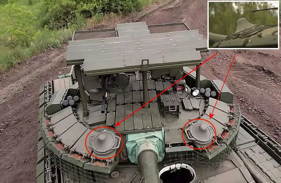
The Breakwater (“Volnorez” / “волнорез” in Russian) electronic protection system was unveiled at the ARMY2023 show in Moscow last year. The size of a dinner plate and weighing 28 pounds, Breakwater attaches to the side of a tank or other vehicle with magnets, providing instant protection. Such devices are sometimes called ‘mushrooms’ or ‘tank boobs.’

The Breakwater creates an invisible 360-degree bubble of protection claimed to extend out to 600 – 1,000 metres, making it far more effective than ‘trench jammers’ which only work out to 50 metres and may not stop an FPV diving towards a target. It can be switched to jam any of twenty different channels commonly used to control drones. But each Breakwater only jams one band, so several may be needed.

According to one Russian military blog

“After being exposed to interference, most drones either veer off course, crashing into the ground, or remain stationary, marking time until they regain signal or run out of energy.”

Generating this protection takes some power, around 70 watts, of which 30 watts is broadcast as radio waves. To provide continuous protection Breakwater has to be installed on a vehicle with an auxiliary power unit; older models like the T-72 do not have one, so the system only works when the engine is on. The protection is blocked by metal, so tanks may have two or more Breakwaters to eliminate any dead zones.

Such jammers are widely sold online on Russia, and bought by charitable groups who send supplies to troops at the front.

You can buy a Breakwater here for 350,000 Rubles or about $3,800. But you might want to hear about one disgruntled buyer’s experience first.

Zero Stars, Do Not Buy

“Romanov Lite” is a Russian military blogger with over 100,000 followers on his Telegram channel, and who carries out frequent fundraising drives for medical supplies and protective gear for soldiers on the front line. And he was not happy with Breakwater.

“Soldiers who received these products are recommended to test them in the field, the results will not please you,”

he advised in a Telegram post, before giving more details of the problems he had found after taking one apart.

First of these was the standard of construction, – the device had clearly been assembled hastily with little or no quality control.

“Absolutely poor build quality. The impression is that the Chinese are soldering all this somewhere in the garage. Therefore, the mean time between failures is the same as in children’s transistors,”

wrote Romanov Lite.

Then there was, perhaps unsurprisingly, the evidence that the device was grossly overpriced in relation to its component parts.

“With a selling price of 350 thousand Rubles ($3800), its real price does not exceed 50 – 60 thousand ($540-$650).”

These should not have come as a shock. Overcharging for poorly-assembled devices made of cheap commercial electronics is pretty much standard in the Russian defence industry. But this jammer had some more fundamental design flaws too.

“The antenna creates a completely open “funnel” above the Breakwater, which Ukrainians spoke about,” says Romanov Lite.

The issue seems to be that the antenna does not, as stated, give full spherical coverage, but more of a toroidal or donut shape. If the opponent is aware of this blind spot — and it seems the Ukrainians are—they can use it to attack from a suitable angle.

There is a worse problem though.

“[In] A violation of all the laws of physics, the transistor module is located in a sealed container ABOVE the cooling radiator, where there is simply nowhere for heat to dissipate and by default it is doomed to burn out, which it does regularly ”

says Romanov Lite.

As noted above, Breakwater consumes 70 watts, converting 30 watts in radio waves; the other 40 watts are dissipated as heat. Managing excess heat is a common issue with electronics, which is why many desktops and laptops have cooling fans and smartphones in insulating cases may overheat.

The Breakwater’s radiator, which is supposed to disperse waste heat into the environment, is located in the heart of the device, so it just recirculates it instead. Even in a Ukrainian winter, the heat is enough to burn out the unit. Bad news for the tank crew, but potentially good news for the makers who can sell another unit, assuming the crew survive long enough to get one.

Follow the Money

These views were echoed by DanielR, a physicist who analyses Russian military hardware on Twitter/X ,

“When I started looking at these photos I was initially very confused as nothing made sense,” DanielR told Forbes. “This is because the quality was much worse than I had expected. “

DanielR was looking at pictures posted by “Serhii Flash” a Ukrainian electronics warfare expert who had dismantled a Breakwater and put his own scathing review online.

“Overall, the quality is more like an electronic toy or home appliance,”

says DanielR, who doubts that the flimsy device held together with sealant and nylon screws would survive for long on a tank.

In his critique, DanielR notes that the DC-DC power converter is a $10 consumer model that is inadequate for the job, and suggests that this is the part which is most likely to fail.

“It seems that someone is making a lot of money,” says DanielR.

Romanov Lite has promised to visit the factory where Breakwaters are made. But if this company disappears, another just like will likely take its place. There is a market desperate for drone jammers, and in the Russian defence business, that means money for crooks.

Source: Forbes

 

armyrecognition.com

Russia Unveils Portable Tank-Mounted Drone Jammer to Counter Ukrainian Attacks | weapons defence industry military technology UK | analysis focus army defence military industry army

---

---

In the ever-evolving landscape of modern warfare, the use of drones has become increasingly prevalent, posing significant threats to armored vehicles on the battlefield. Responding to this emerging challenge, Russia has unveiled its latest countermeasure, the REB "Волнорез" (Volnorez - Breakwater) electronic warfare jammers. This state-of-the-art system was first showcased and mounted on a T-80BVM Main Battle Tank (MBT) during the Russian Army Expo 2023 defense exhibition, capturing the attention of defense analysts worldwide.
Follow Army Recognition on Google News at this link

---

The Russian-made Volnorez portable drone jammer system can be easily mounted on a tank turret to counter drone attacks. (Picture source Facebook Garupan History)

---

The Volnorez boasts impressive frequency coverage, spanning from 900 MHz to 3,000 MHz. This wide spectrum ensures that it can effectively jam a variety of drones operating within this range. With the ability to disrupt drone signals from over a kilometer away, the Volnorez stands as a formidable deterrent against aerial threats. Once jammed, most drones either veer off course, crashing into the ground, or remain stationary, loitering in place until they either regain signal or deplete their power reserves. This capability ensures that vehicles equipped with the Volnorez, as well as those in its vicinity, gain a significant layer of protection against drone attacks, marking a game-changer in defensive capabilities, especially in conflict zones like Ukraine.

One of the standout features of the Volnorez is the versatility of its jammer antennas. These are magnetically attached, allowing for flexible placement on almost any part of the vehicle. Furthermore, the jammer signals are omnidirectional, ensuring 360° of protection regardless of the antenna's position on the vehicle. While it's believed that the Volnorez is primarily fitted on vehicles equipped with an auxiliary power unit (APU) to ensure uninterrupted operation, early tests of the system were conducted on a T-72B3 tank, which did not have an APU. This suggests potential versatility in its deployment across different vehicle platforms.

The introduction of the Volnorez jamming system underscores the importance of electronic warfare in modern combat scenarios. As the situation in Ukraine continues to evolve, the effectiveness of this new system will undoubtedly be closely watched by military experts and strategists around the globe.

---

Defense News September 2023

 

3-D High-Resolution ISAR Imaging for Noncooperative Air Targets | IEEE Journals & Magazine | IEEE Xplore

ISAR image of the PZL KR-03 Puchatek.

3-D High-Resolution ISAR Imaging for Noncooperative Air Targets | IEEE Journals & Magazine | IEEE Xplore

Marcin Kamil Baczyk; Piotr Samczynski; Jedrzej Drozdowicz; Maciej Wielgo; Jakub Sobolewski; Marek Ciesielski; Jakub Julczyk

ieeexplore.ieee.org

Abstract:This article uses the inverse synthetic aperture radar (ISAR) imaging method to present real-world tests on 3-D radar imaging of noncooperative air targets. Initially, th...View more

Metadata

Abstract:

This article uses the inverse synthetic aperture radar (ISAR) imaging method to present real-world tests on 3-D radar imaging of noncooperative air targets. Initially, the fundamentals of 3-D ISAR are introduced. This is followed by a discussing of the challenges of obtaining high-quality 3-D radar images. An essential feature of the applied method is its basis on the back-projection family of techniques, eliminating the need for iterative image reconstruction. These theoretical concepts are validated using both simulations and real-life signals. This article also provides insights into the measurement campaign and the signal processing techniques applied to achieve the presented results.

Page(s): 4194 - 4207

Date of Publication: 23 January 2024

Figures are not available for this document.

---

In The modern battlefield, air target imaging and classification are crucial tasks. The primary sensors used for these purposes are optical and radar sensors. The advantage of optical sensors is their high resolution; however, the disadvantage is their high dependence on weather conditions, such as fog, cloudy weather, rain, snow, or image dispersion due to air temperature differences. Lower resolutions to the optical images characterize radar imaging. However, it allows the creation of a target image independently of the weather conditions, enabling day and night operation. The resolution of the radar imaging depends on the bandwidth of the emitted signal. Nowadays, a centimeter resolution is easily achievable using GHz and more bandwidths [1], [2], [3], [4], [5], [6], [7]. Such a resolution is sufficient regarding air target classification [8], [9], [10], [11]. The inverse synthetic aperture radar (ISAR) technique, developed in the last century [12], [13], is most often used for the radar imaging of air targets. The 2-D ISAR has now entered the maturity stage, which can be seen in various advanced and highly efficient methods, e.g., [14], [15], [16], [17], [18], and [19]. Over recent years, many different demonstrators of this technology have been developed, and the 2-D ISAR has also been implemented in final radar products offered by the industry [20], [21], [22].

As 2-D ISAR imaging is a mature technology, in recent years, researchers have been focusing on novel 3-D ISAR imaging techniques [23], [24], [25], [26]. Up to now, 3-D radar imaging has been used mainly in the remote sensing applications of Earth imaging, where the interferometric synthetic aperture radar (InSAR) method has been applied [27], [28], [29], [30], or in tomography imaging [31]. The 3-D ISAR also uses the same interferometric approach as InSAR. The main difference is in geometry. Recent studies show that 3-D ISAR imaging is feasible [32], [33], [34], [35]. However, in most cases, the validation has been obtained by simulation [32], [33], or using huge targets, such as ship-borne targets [36] with relatively low resolution. To the authors' knowledge, there is no evidence of high-resolution 3-D ISAR imaging of noncooperative air targets based on real measurement. Such imaging is challenging and requires much more effort than in the simulated control environment, where the algorithm fully knows the target trajectory.

In recent years, several studies have emerged focusing on 3-D ISAR imaging. A common approach found in numerous publications involves deploying three receiving antennas arranged in two orthogonal baselines [32], [37], [38], [39]. This configuration facilitates interferometry in both directions, paving the way for a straightforward acquisition of 3-D imagery. Typically, 2-D imaging in these methodologies is achieved using the range–Doppler (RD) technique, which, while widely adopted, has inherent limitations concerning velocity and range resolutions. Several other methods for obtaining 3-D imagery have been proposed in literature, including the polar format algorithm (PFA), which the authors delve into in this work [40]. While some researchers have suggested employing just two receivers for 3-D imaging, the detailed mechanics of transforming the interferometric amplitude and phase data into 3-D images often remain inadequately elucidated [41], [42].

This article presents new results of developing the multichannel ground-based radar demonstrator allowing for high-resolution 3-D ISAR imaging of noncooperative air targets with a 15-cm resolution range. Contrary to approaches in literature, the proposed one uses only two receiving antennas for 3-D ISAR imaging. The system has been developed within the 3-D radar imaging for the noncooperative target recognition (RING) project. The RING project is a research and technological development project funded by the Italian and Polish Ministries of Defence and carried out for the European Defence Agency (EDA) in 2019–2023. The RING project focuses on developing and validating novel 3-D ISAR imaging techniques and novel noncooperative target recognition (NCTR) algorithms for this technology. The authors believe that the results of the RING project would be a game changer in the future of radar-based systems for target classification and recognition [43].

The main contribution of this article is the InISAR processing adopted for high-resolution noncooperative 3-D target imaging. The novelty can be summarized as follows.

1. The back-projection algorithm (BPA)-based approach was adopted for 3-D ISAR imaging using two receiving antennas.

2. The problem of trajectory estimation for high-resolution radars was addressed.

3. Extensive simulation experiments were carried out to confirm the method's usability.

4. Practical experiments, including the 3-D high-resolution imaging of noncooperative targets in a real-life scenario, were conducted.

The authors want to highlight that the whole article can be treated as a comprehensive tutorial guiding through principles, simulations, practical implementation, and measurement.

The rest of this article is organized as follows. Section II presents the theoretical background of 3-D ISAR imaging. In Section III, the authors present the simulation results of noncooperative targets' proposed 3-D high-resolution imaging. All the processing stages of the algorithm are explained step by step, showing the main challenges and solutions for correctly processing the data to obtain high-resolution and high-quality 3-D ISAR imaging of the noncooperative air targets. In addition, the challenges in signal processing for 3-D ISAR image creation of noncooperative targets with unknown trajectories are discussed in detail. In Section IV, the comparison to other 3-D imaging methods was presented. Then, Section V shows the real-life signal analysis results. In addition, the architecture of the developed high-resolution radar operating in the X-band and the first real-life results of the 3-D ISAR imaging of a noncooperative air target were obtained using records from the developed radar demonstrator. Finally, Section VI concludes this article.

SECTION II.

Theoretical Background

A. Signal Model

Range resolution (δr) in monostatic radar results from signal bandwidth (B) according to the following relationship:

δr=c2B(1)

View Sourcewhere c is the speed of light. High cross-range resolution can be achieved through the application of ISAR processing, which synthesizes a radar aperture to capture the movements of the target over a substantial integration time.¹ This results in variations in the Doppler frequency of the radar echoes that are reflected off the target's different components.

For this study, the point reflectivity model was utilized for analysis. While the authors fully acknowledge its limitations and potential deviations from real-world scenarios, it is pertinent to note that this model offers a reasonable approximation under constrained integration times and operation in the far-field region. Therefore, given these specific conditions, the employment of the point reflectivity model is deemed appropriate for the presented research objectives.

One of the simplest ways to obtain a high-range resolution of SAR or ISAR systems is to use linear frequency-modulated (LFM) signal pulses. A single LFM pulse is defined as

stx(τ)=rect(τTp)⋅exp(j2π⋅(fcτ+γτ22))(2)

View Sourcewhere j=−1−−−√, rect(⋅), and exp(⋅) represent rectangular and exponential functions; and Tp, fc, and γ denote pulse time width, carrier frequency, and chirp rate, respectively. To obtain an image, multiple pulses are emitted with pulse repetition interval (PRI) time Ti=1fPRF, where fPRF is the pulse repetition frequency (PRF).

Assuming stop-and-go approximation, the received echo signal reflected from K scatterer centers can be expressed as

srx(t,tn)=∑k=1Kσk⋅stx(t−rk(tn)c)(3)

View Sourcewhere t and tn=nTi denote so-called fast and slow time, and σk and rk(tn) denote the scatterer coefficient and the range of the kth target point.

The use of the LFM waveforms allows for significantly reduced effective signal bandwidth. After the application of the dechirp method (matched filtering in the time domain), the received signal can be presented as

sr(t,tn)==srx(t,tn)⋅s∗tx(t)rect(tTp)∑k=1Kσk⋅exp(−j2πfcrk(tn)c)⋅exp(−j2πγtrk(tn)c)⋅exp(j2πγ2(rk(tn)c)2).(4)

View SourceThe last term in (4) is the residual video phase and can easily be removed after the pulse compression procedure [44].

The model presented above (4) works for the pulsed and continuous wave (CW) radars using LFM signals. In the case of frequency-modulated continuous wave (FMCW) radar in the model (2), t=Tp in rect(tTp) which means that the duty cycle equals 100%. The FMCW radar has been referred to here, as nowadays, this kind of radar allows one to achieve wideband illumination with relatively low costs. Analog-to-digital converters (ADC) with lower sampling rates and a higher number of bits can be used to sample the beat signal compared to the pulse radar, where the whole bandwidth needs to be covered. In the case of achieving 15cm-resolution in range with 1-GHz bandwidth, in the case of pulsed radar, ADCs with at least 2-GHz sampling frequency have to be used; as for FMCW, a sampling frequency in the tens of MHz is usually sufficient. The authors have developed this kind of radar demonstrator within the work presented in this article, and further analysis will be made for the case of the FMCW radar. However, the model presented in the article also works for the pulse radar.

In the FMCW radar, according to (2), each moment can be assigned to the instantaneous frequency (beat signal) of the emitted signal. Therefore, by changing the coordinates in (4), it can be represented as follows:

sr(ft,tn)=rect(ftB)∑k=1Kσk⋅exp(−j2πfc+ftcrk(tn))(5)

View Sourcewhere ft=γt denotes the current frequency in baseband.

The signal model given by (5) represents the cross-power spectrum density of the transmitted and received signals. It is worth noting that this form of the received signal does not consider the duration of a single pulse. This is simply due to the assumption that the scene is stationary for a single range profile evaluation.

B. Scene Geometry

Term rk(tn) appearing in (3)–​(5) denotes the range of the kth scatterer from the transmitting and the receiving radar antennas. Despite the short distance between antennas and, therefore, the monostatic configuration of the radar scene, a bistatic model of the range between the target and the radar can be applied. This has to do with the interferometric approach, where multiple receiving antennas have to be used to obtain the 3-D model of the target. The scene's geometry for 3-D ISAR imaging is shown in Fig. 1. In the case of the presented interferometric radar, the receiving antennas are located directly above the transmitting antenna at a short distance.² Notations from Fig. 1 can be summarized as follows:

1. rk,1(tn)—Represents the position of a specific point with respect to the transmitter.

2. r1(tn)—Denotes the position of the object's centroid with respect to the transmitter.

3. rk,2,1(tn)—Represents the position of a specific point with respect to the first receiver.

4. r2,1(tn)—Denotes the position of the object's centroid with respect to the first receiver.

5. rk,2,2(tn)—Represents the position of a specific point with respect to the second receiver.

6. r2,2(tn)—Denotes the position of the object's centroid with respect to the second receiver.

7. rPk(tn)—Signifies the position of a particular point relative to the object's centroid.

8. v(tn)—Represents the velocity of the object.

In the presented model, the observed target moves in a straight line at an established range from the radar at a fixed height. The target's position in the global coordinate system is expressed by rtrg(tn). In addition to the target's position, its orientation relative to this frame of reference is essential. The Tait–Bryan angles denote the vector eatrg(tn)=[Ψ(tn)Θ(tn)Φ(tn)]T, where successive elements represent the rotation of the target along corresponding axes.³

Let Pk denote a scatterer whose location relative to the target's center is given by rPk(tn). In addition, let the value of the rPk vector be expressed in the coordinate system associated with the observed target O′X′Y′Z′. In this system, the position of scattering point Pk does not change in time, regardless of the location of the target rtrg(tn) and its spatial orientation eatrg(tn). It was assumed that the target might be treated as a rigid body.

In the case of determining radar imagery, it is important to determine how the range of a given scattering point from the transmitting and mth receiving antenna varies in time

rk,m(tn)=∥rk,1(tn)∥+∥rk,2,m(tn)∥.(6)

View SourceThis value called the bistatic range, is expressed as the sum of the lengths of the vectors defining the position of a given scattering center to the transmitting and the mth receiving antennas, which are given by the following formulas:

rk,1(tn)=rk,2,m(tn)=r1(tn)+Mrot(eatrg(tn))rPkr2,m(tn)+Mrot(eatrg(tn))rPk(7)

View Sourcewhere Mrot(eatrg(tn)) denotes the rotation matrix by the Tait–Bryan's angles defined by target orientation eatrg(tn).

The object's orientation vector eatrg(tn) is estimated based on its trajectory. It is important that, contrary to other procedures, the rotation vector is not directly used for imaging purposes. Instead, it provides an essential context for understanding the object's orientation and potential movements during observation.

The coordinate system will be associated with the center of mass of the observed target Otrg to become independent of its local orientation. In this way, the observed target remains in the center of the coordinate system. The transmitting and receiving antennas circulate the target according to a fixed trajectory depending on the target's position and orientation in the global coordinate system. Therefore, the position of the target to the transmitting and receiving antennas should be redefined

r1(tn):=r2,m(tn):=Mrot(−eatrg(tn))r1(tn)Mrot(−eatrg(tn))r2,m(tn).(8)

View SourceThe trajectory parameters defined by (8) allow for adopting a geometry adequate for the SAR scenario but in inverse geometry in the case of ISAR imaging. This approach is not required but allows for simplifying (5).

C. 2-D High-Resolution ISAR Imaging

Over the years, many methods have been developed to determine 2-D SAR/ISAR images [44]. The most accurate methods with minor distortion are based on the BPA. In general, it simulates the radar response of a given point with a predetermined target trajectory. The simulation result correlates with the registered signal to estimate the coefficient σk at a given scattering point. The above procedure is repeated for all points positions of the image to be determined.

The main disadvantage of the BPA [45], which precludes its use in real time in practical applications, is the number of calculations required to determine the final image. The computational complexity of such an algorithm is O(n3). In particular, high-resolution images with enormous pixels require high computational capability. For this reason, in the presented approach, the PFA has been proposed [46]. The PFA method can be perceived as an example among several algorithms that stem from the BPA methodology. The PFA can also be regarded as a computationally efficient variant of BPA, taking into account specific simplifications and inaccuracies. The choice to leverage PFA in later sections was driven by these computational benefits while preserving the BPA methodology's core principles. This approach takes advantage of the fact that for small and distant targets, it is possible to approximate expression (6) with an appropriate dot product. Assuming r1(tn)≫rPk and r2,m(tn)≫rPk, the corresponding ranges may be expressed as

rk,1(tn)≈rk,2,m(tn)≈r1(tn)+r^1(tn)∙rPkr2,m(tn)+r^2,m(tn)∙rPk(9)

View Sourcewhere • denotes the dot product operator, and r^1(tn)=r1(tn)r1(tn) and r^2,m(tn)=r2,m(tn)r2,m(tn) represent unit vectors of the same direction as r1(tn) and r2,m(tn), respectively.

Substituting (9) and (6) into (5) and after rearranging terms, the signal received by the mth receiving antenna takes on the following form:

sr,m(ft,tn)=rect(ftB)⋅exp(−j2πfc+ftcrm(tn))⋅∑k=1Kσk⋅exp(−j2πfc+ftcr^m(tn)∙rPk)(10)

View Sourcewhere

r^m(tn)=r1(tn)r1(tn)+r2,m(tn)r2,m(tn)(11)

View Sourcecorresponds to the direction in which the radar observes the target.

This short method description does not consider any positioning or orientation errors and their influence on final results. Since the target trajectory is assumed to be known, it can easily be removed from the received signal

sr,m(ft,tn)=∑k=1Kσk⋅exp(−jkm(ft,tn)∙rPk)(12)

View Sourcewhere km(ft,tn)=2πfc+ftcr^m(tn) denotes wave vector. After resampling (12) in the spatial frequency domain associated with the vector k, the scattering coefficient σk can be estimated using the inverse Fourier transform. Due to the efficient implementation of this algorithm, the computational complexity of PFA is much lower than the traditional BPA approach.⁴

D. 3-D Projection Onto a 2-D Plane

Typically, with SAR/ISAR processing, the generated image is 2-D. The imaging plane can be chosen in any way, but the best results are obtained when the plane is the same as the O′X′Y′ plane (greyed area in Fig. 1).

The determined scattering coefficients correspond to the appropriate points on the plane for which the imaging is determined. It is worth noting that every scattering center of the observed target that does not lie on this plane will also be imaged. It is practically impossible to distinguish the image of a point located on the imaging plane from the image of a point below or above this plane when using data recorded with only one transmitter–receiver pair.

The point at which the image of a scattering center not lying on the imaging plane will be located depends on the relative position of the transmitting and receiving antennas, the observed target, and its direction of movement. Of course, due to the changing geometry of the scene, for a sufficiently long integration time, points not lying on the imaging plane will not be focused. However, relatively short integration times are used for a wideband radar with a high carrier frequency. Therefore, it can be assumed that the scene's geometry does not change so much that the images of points not lying on the O′X′Y′ plane are unfocused.

Two points will be identical on the image if they have the same bistatic parameters. Relative to the target center, the bistatic range can be defined as

Δrk,m(tn)=r^m(tn)∙rPk.(13)

View SourceSimilarly, relative bistatic velocity can be defined as

Δvk,m(tn)=∂Δrk,m(tn)∂tn=d^m(tn)∙rPk(14)

View Sourcewhere

d^m(tn)=v(tn)−(r^1(tn)∙v(tn))r^1(tn)r1(tn)+v(tn)−(r^2,m(tn)∙v(tn))r^2,m(tn)r2,m(tn).(15)

View Source

In this context, the parameter d^m(tn) is derived based on the object's trajectory and can be treated as an effective single rotation vector for the entire object. This value is then determined for a point representing the object's centroid.

Let P′k,m denote a point lying on the imaging plane whose projection on the image obtained for the mth receiving antenna is the same as point Pk. Therefore, the following linear system can be written:

{r^m(tn)∙rP′k,m=r^m(tn)∙rPkd^m(tn)∙rP′k,m=d^m(tn)∙rPk.(16)

View Source

Generally, the position rPk of the point Pk is defined in 3-D Cartesian coordinates. There are infinite points Pk satisfying (16). Additional measurements are necessary to determine the exact position of the scattering center.

E. Interferometry-Based 3-D Imaging Technique

One way to achieve 3-D imaging is to use interferometry. This method is generally based on information about the phase of the estimated scattering coefficient of the imaged target's point.

If the antenna array of the radar system is calibrated, the phase of the received signal should not change during the imaging procedure. When a reflecting point has a real-value reflectivity value, the estimated reflectivity value of the scattering center should also be a real-value number. However, this statement only holds if the scattering center is located precisely on the grid, at the position where the value is determined. Therefore, the estimated single scattering point reflectivity may have shifted phase in complex value reflectivity. The phase change of the determined value depends on the wavelength of the signal used to illuminate the target and the difference in the distance between the actual position of the point image and the grid point representing the given point.

In the case of the interferometry technique, the fact is that for two receiving antennas located at different heights, the projection position of a given point on the imaging plane will be different. This results directly from (16). With a slight difference in the position of the antennas, it can be assumed that the difference in the position of the projected point rP′k,m on the imaging plane for both receiving antennas is significantly smaller than the size of a single range cell. This can be written using the following align:

∥∥rP′k,1−rP′k,2∥∥≤δr10(17)

View Sourcewhere δr is the range resolution of the radar system.

The range expressed by (13) denotes the bistatic⁵ range of a given scattering center in relation to the bistatic range of the target's center. In this expression, the compensation of the range of the target from the radar is considered, which ensures that it has no direct effect on the image formation process. The value given by this expression is the length of the vector, being the projection of the vector rPk on the line whose direction is given by the vector r^m(tn). Since the value given by (13) denotes the difference in the relative ranges of a given point rPk from the radar for different receiving antennas, it can be stated that

(r^2(tn)−r^1(tn))∙rPk=λcϕ2−ϕ12π(18)

View Sourcewhere ϕm denotes the phase of the estimated scattering coefficient of the mth image and λc denotes the wavelength of the signal illuminating the target.

Combining (16) and (18) into a single equation system, the following expression can be stated

ArPk=b(19)

View Sourcewhere A=⎡⎣⎢⎢r^1(tn)Td^1(tn)T(r^2(tn)−r^1(tn))T⎤⎦⎥⎥ and b=⎡⎣⎢⎢⎢r^1(tn)∙rP′k,1d^1(tn)∙rP′k,1λcϕ2−ϕ12π⎤⎦⎥⎥⎥. Resolving (19), position rPk can be directly estimated.

F. 3-D Reconstruction Analysis

In 3-D ISAR imaging, the solution vector rPk is derived from (19). A necessary condition for an accurate estimation of rPk is the invertibility of matrix A.

The invertibility of matrix A is fundamentally tied to its determinant, with the nonzero determinant being a prerequisite for inversion. A determinant approaching zero is symptomatic of linear dependence between the matrix's rows or columns.

For matrix A, linear dependence between its columns typically implies that one of the coordinates is not represented in the data. This situation often arises when the object's motion and the distribution of receiving antennas lie within the same plane. Conversely, linear dependence among rows indicates scenarios where the object moves along the line of sight (LOS), manifesting parallelism between vectors r^1(tn) and d^1(tn), or when receiving antennas are positioned along the direction defined by LOS, which leads to parallelism between vectors r^1(tn) and r^2(tn)−r^1(tn).

A detailed analysis of (19) and the precision of determining the 3-D point's location exceeds the scope of this article. Here, the authors merely wish to highlight situations where matrix A is noninvertible, precluding proper 3-D imaging. The cases directly indicated by the invertibility requirement of this matrix align with the intuitive understanding underlying interferometry.

Since interferometry is not fully 3-D imaging, additional assumptions about the nature of the target are necessary. First, there cannot be two points with the same projection onto the imaging plane. Otherwise, those two points will interfere, and the estimated phases ϕ2 and ϕ1 will be distorted. Second, the target displacement during integration time due to approximations used in (13) and (14) are no longer valid. It is worth noting that using mechanisms based on interferometry is necessary to ensure that both of the above conditions are met. Otherwise, the presented technique may return improper results.

SECTION III.

3-D Imaging Verification via Simulations

Many simulations were conducted to verify the mechanism for determining the 3-D imagery described in Section II. A block diagram presented in Fig. 2 shows the verification procedure for a single azimuth angle. Initially, the direction of the object's motion was selected. Subsequently, the target trajectory was generated, and a simulation of the object's echo was conducted. In the following stages, a 2-D image was created, interferometry was determined, and a 3-D reconstruction of the simulated object was carried out. The final step involved comparing the estimated positions of the object's points with those simulated. Representative results are presented in the next section.

Fig. 2.

Block diagram of presented 3-D ISAR processing verification method.

Show All

A. Simulation Setting

A simplified model of the KR-03 Puchatek glider consisting of 117 points was used. The model can be seen in Fig. 3. The simulated target is similar to that used in the real-life experiment described in detail in Section V. The simulated object was moving 100m from the radar at an altitude of 30m at a speed of 30 m/s. This scene can be seen in Fig. 4. The transmitter was at point [000] m, and the receivers were at points [010] m and [020] m. The carrier frequency and the bandwidth of the simulated signal were 10 and 1GHz, respectively. The presented parameters of the scene and signal correspond to the parameters of the conducted measurement experiments described in the further part of this article.

B. Range–Doppler Map Evaluation

To verify the performed simulations, RD maps were evaluated. Fig. 5 is a reference for other images for better intuition and understanding of the imaged target and scenario. It shows the difference between the RD and the considered techniques.

Fig. 5.

RD maps for two time instants (integration time was s0.1). (a) T= s1.1. (b) T = s3.4.

Show All

RD imaging is numerically thrifty; no input parameters, like trajectory, are required. As can be seen, the glider shape can be distinguished in the picture; however, the quality is low, and the image is tilted. Based on RD imaging, 3-D reconstruction might need to be more precise. More complex imaging algorithms are recommended for high-resolution imaging.

C. 2-D Imaging

In Fig. 6, a 2-D ISAR image obtained using the PFA algorithm can be seen. The scatterers can be distinguished due to much higher imaging resolution compared to Fig. 5. For example, the image contrast of results presented in Fig. 6 equals 3.48 versus 1.61 and 1.85 of images shown in Fig. 5(a) and (b), respectively. However, it is impossible to obtain information about the elevation profile. It is worth noting that, in this case, the tail wing above the imaging plane is shifted in the positive direction of the OY axis. This shift results from the simple fact that elements above the imaging plane are slightly more distant from the radar than corresponding elements on this particular plane in the simulated scenario. Fortunately, this shift does not noticeably blur these points in the image, and almost all scattering centers can be identified.

Fig. 6.

ISAR image of the simulated target for the PFA algorithm.

Show All

D. Interferometry and 3-D Imaging

The phase difference, shown in Fig. 7, was determined based on complex 2-D imaging values for different receivers. The color indicates the value of the phase of the estimated scattering coefficient whose amplitude, shown in Fig. 6, is greater than −20dB.

Fig. 7.

Phase shift for interferometric measurements.

Show All

The graph presented in Fig. 7 is not a typical 3-D image, but on its basis, it is possible to determine the altitude profile of the observed target. It is worth paying particular attention to the phase value of the points in the fuselage area. The darker areas, corresponding to lower points, are shifted in the negative y-axis direction. On the other hand, the brighter ones, corresponding to higher points, are shifted toward the positive values of the OY axis. Nevertheless, in the adopted model, shown in Fig. 3, all hull points have the y coordinate equal to 0. Similarly to the shift described in Section III-C, this results from the different ranges of those areas from the transmitting and receiving antennas and is the basis of the 3-D interferometric imaging technique.

Finally, the 3-D ISAR imaging described in Section II is conducted. Fig. 8 shows the result. In the 3-D image, points making the glider can be distinguished and presented as blue circles. The radius of the circle corresponds to the amplitude of the scattering point.

Fig. 8.

Comparison of reconstructed target and the simulated one.

Show All

E. Simulation Conclusions

The results presented in this section prove that the proposed methods work correctly. 3-D interferometric images can be obtained with sufficient quality. Fig. 8 presents the 3-D target reconstruction. The average distance of the reconstructed target's estimated points from the points of the simulated model is not more than 0.25m. This result is satisfactory considering the image resolution of 0.15m.

In addition, simulations were carried out for different directions of the target's motion relative to the LOS. Fig. 9 shows the average distance of all estimated points of the reconstructed target from the points of the simulated model as a function of the target's azimuth. The lowest values are obtained when the target moves in the direction perpendicular to the LOS. This direction in the simulation corresponds to an azimuth of 90∘.

Fig. 9.

Reconstruction performance in function of target moving direction.

Show All

What is important to note is that this data processing approach works well on simulated data, where an exact trajectory can be used. Additional procedures that prepare and process data must be used to process real-world data. Implementing those procedures and finding adequate algorithms is one of the main difficulties in 3-D ISAR interferometric imaging. Those procedures, problems, and mitigations are described in the next section.

SECTION IV.

Comparison to Other Methods

In 3-D ISAR imaging, existing techniques often rely on the RD algorithm, which typically requires at least three receiving antennas to accurately reconstruct a 3-D image of a moving target. However, the proposed method offers a significant advantage: it can generate high-quality 3-D images with only two receiving antennas, which reduces system complexity, dimensions, costs, and weight. By requiring fewer receiving antennas, the proposed method offers potential cost savings. It simplifies the imaging setup, making it more accessible for various applications and easy to deploy in demanding locations.

While ISAR imaging is a well-established method for generating high-resolution 3-D images of moving targets, many existing techniques rely on the CLEAN algorithm to separate the target from the clutter in the resulting image. However, this approach can be computationally intensive and limit the imaging process's speed and efficiency. In contrast, the proposed method simultaneously processes the pixels of the entire image, which offers several benefits. The presented technique reduces the computational complexity by analyzing the entire image in one step. It speeds up the imaging process, making it more efficient and practical for real-world applications. Furthermore, the proposed approach avoids the limitations of traditional CLEAN-based techniques, which can struggle to reconstruct targets with complex shapes accurately or in scenarios with significant interference.

The 3-D target reconstruction results obtained using the CLEAN technique are presented in Fig. 10. The reconstructed target model generally fits well with the target model used in the simulation, and the number of scatterers is estimated accurately with this method. However, it is important to note that the CLEAN technique is computationally intensive, requiring more than 100 evaluations of the imaging and simulating processes to generate the final image.

Fig. 10.

comparison of reconstructed target and the simulated one for CLEAN technique.

Show All

While the CLEAN technique is a powerful tool for ISAR imaging, it has some limitations, mainly when dealing with dense reflectivity functions. The problem arises when the target contains complex features or is located in an environment with high interference levels, leading to a dense reflectivity function.

It is essential to clarify that the presented analysis does not explicitly enumerate the required computational operations, as this is inherently contingent upon the selected imaging methodology. In this study, the authors advocate for the PFA method, renowned for its computational efficiency in image derivation. It is noteworthy, however, that alternative strategies, such as the classic back-projection, are equally viable. The discourse primarily underscores the merit of processing the complete 3-D image in a consolidated step. This stands in contrast to iterative techniques like CLEAN, which tend to extract individual reflecting points repetitively. From the presented analysis, this comprehensive approach to image processing provides a more integrated and holistic representation, surpassing the granularity offered by conventional point extraction methodologies.

SECTION V.

Real Data Measurement Description

Section III outlined the signal processing chain using simulated data. It should be noted that processing real-life signals is significantly more challenging than simulated data. This is mainly due to the adopted models of physical phenomena and the assumption of ideal conditions.

This section presents the processing of signals recorded during experiments with a real target. Particular attention was paid to the aspects affecting the final result's quality. These issues include, first of all, the estimation of the trajectory and spatial orientation of the observed target. Generally, the relative accuracy of the range evaluated should be lower than the fraction on wavelength, which in the case of X-band radar is less than 1cm. Thus, this section is dedicated to 3-D ISAR imaging and trajectory estimation and its enhancement for real-life ISAR imaging.

Fig. 11 presents a block diagram of the processing algorithm adapted to measurement data. An essential part of the presented algorithm is classical radar processing, which leads to detecting and tracking the observed target. Thanks to this, it is possible to extract the desired target echo from the recorded signals and process it following the procedure presented in Sections II and III.

Fig. 11.

3-D ISAR processing block diagram.

Show All

A. FMCW Radar Demonstrator

An FMCW radar with one transmitting and four receiving channels was used during the measurement campaign. An example of an antenna array of the X-band system is presented in Fig. 12. The horn antennas used during the experiment cover the frequency band from 8.5 to 11.5GHz. Table I lists the rest of the system's parameters.

TABLE I Demonstrator Parameters

Fig. 12.

Antennas setup of the X-band active radar demonstrator.

Show All

During the measurement campaign, the system could register echo signals for up to four antennas, and all data recorded were processed. However, in obtaining 3-D imaging, only data from two of those antennas were used. This approach is consistent with the initial proposition, underscoring the core methodology.

B. Measurement Campaign and Data Acquisition

The observed target was a KR-03 Puchatek glider shown in Fig. 13. It was on its final approach for landing. The target was moving at constant forward and vertical speeds.

Fig. 13.

PZL KR-03 Puchatek glider.

Show All

The Puchatek glider used for method validation is relatively big compared to general aviation aircraft and is mainly made of metal, which provides good SNR. The Puchatek has a wingspan of 16.4m, a length of 8.63m, and a height of 1.55m. Usually, it flies at speeds lower than 35 m/s, which mitigates velocity unambiguously.

C. Signal Conditioning and Clutter Filtering

The method presented in Section II is based on the assumption that the signal is transmitted and received at the antennas' points. In a real-world scenario, the analog front end (AFE) induces additional delays and distortions that must be compensated. In the presented work, this process, called signal conditioning, is based on estimating the parameters of the first echo caused by antenna leakage.

After signal conditioning, strong echoes of stationary objects are removed by low-pass filtering. The finite impulse response (FIR) filter with a sufficiently long pulse response allows one, on the one hand, to keep the echo of the target close to zero-Doppler; on the other hand, it removes most of the stationary echoes. As a result of signal conditioning and clutter removal, the SNR increases, and the target can be detected.

D. RD Processing

Relatively high target speeds usually create two serious problems that must be addressed. The first problem is range migration directly caused by the significant velocity. In the case of radars with 15cm-range resolution, the range migration is achieved even at low speeds of the target. Therefore, the 2-D discrete Fourier transform is insufficient to focus the target echo correctly, so the Keystone algorithm was adapted for this purpose. It allows for computationally efficient determination of the RD maps independently of the linear radial velocity.

E. Target Detection and RD Positioning

Before imaging, a noncooperative air target must be detected and tracked first. One of the main challenges of high-resolution radars is precise positioning, which is necessary for ISAR imaging. Assuming a high SNR, the expected accuracy of determining the target's range and velocity should be similar to the resolution of the RD image. Air target positioning with high-resolution radars has not been widely discussed in literature and has yet to be comprehensively resolved.

The adopted algorithm for target position estimation consists of several stages. First, based on evaluated RD maps, the standard constant false alarm rate (CFAR) is applied, and points above the threshold are returned. Then, density-based spatial clustering of applications with noise (DBSCAN) [47] combines a dozen detections into several potential targets.

The actual target range and velocity are estimated by having detections clustered. This results from several observations. At any time, the target is visible from a slightly different angle. Therefore, at each subsequent moment, the echoes of various elements of the observed target may dominate the recorded signal, and the classic detection algorithm may return other points. Moreover, the registered echo might be incomplete, which biases the target position's estimation.

The method based on the RD target image's center of gravity was adopted according to the abovementioned difficulties. The target's location r^rv is evaluated as the weighted average of the position of all detections belonging to this target

r^rv=∑jrrv,j|σj|∑j|σj|(20)

View Sourcewhere rrv,j and σj denote the position of the jth RD cell and estimated scatterer coefficient for this cell, respectively.

Fig. 14 shows two extracted echoes of the observed target on the RD maps evaluated for two different moments, together with marked centers of gravity. It is worth noting that there are significant differences in the echo structure, which impedes the proper estimation of the target's center.

Fig. 14.

Detection on RD maps (integration time - s0.1). (a) T= s1.5. (b) T = s3.0.

Show All

F. RD Tracking

Target tracking in radial coordinates is determined in successive moments based on the estimated RD positions. Based on these track parameters, it is possible to decide how the range and radial velocity change over time. Due to the limited possibilities of accurately estimating track parameters, it is essential to estimate the motion model correctly. In this case, the Kalman filter is usually applied and adopted.

Fig. 15 shows the result of radial tracking for individual receiving antennas in different colors. A relatively high variance of the parameters of the estimated tracks can be noticed. The estimated trajectory in this way is unsuitable for evaluating the target position and must be corrected in the next steps.

Fig. 15.

Tracks and estimated trajectory.

Show All

G. Target Extraction

Other echoes of moving targets and noise or interference affect the final processing results. This influence manifests itself primarily in a significantly reduced SNR. Thus, the next critical signal processing stage is extracting the observed target echo from the recorded data.

The trajectory estimated during RD tracking isolates the target echo. The input data are filtered with a 2-D nonstationary bandpass filter. Since the received signal contains only the echo of the observed object, it is possible to significantly reduce the sampling frequency, both in the fast-time and slow-time domains, which additionally reduces computational complexity.

Fig. 16 presents range-slow time maps for extracted target echo. With the red line, the estimated target center is denoted. Based on estimated ranges, accurate target tracking and positioning are further performed.

Fig. 16.

RT map with a superimposed trajectory (red curve).

Show All

H. Cartesian Tracking

Accurate location and target tracking were among the most challenging stages of data processing. The quality of the final result heavily depends on the accuracy of the estimated trajectory. It is important to note that an object with an incorrectly matched 3-D trajectory will likely have a distorted representation. In the case of aerial objects, such as the observed gliders, symmetry is expected. However, this symmetry can be disrupted if the azimuth and trajectory are estimated incorrectly, leading to skewed or unbalanced images.

During the measurements, the antenna array of four antennas was placed at the corners of a rectangle with a side length of 2 m (see Fig. 12). Despite this setup, determining the elevation and azimuth angles of the target with high precision was challenging. Consequently, it was assumed that the observed target, a landing glider, moved in a straight line at a constant velocity. Given the low altitude typically associated with landing gliders, it was further assumed that the target was at a relatively low height. Based on these assumptions, it was determined the target's position in the Cartesian coordinate system using only range measurements.

This approach, centered on simplicity, proved effective for initial trajectory estimation in our experimental setup. The linear motion assumption provided a practical basis for the presented analysis, especially when detailed motion dynamics were either unavailable or unnecessary for the level of imaging the authors sought to achieve. While this method may not capture the complete range of motion dynamics, it offers a foundational understanding of the target's trajectory, sufficient for imaging purposes.

Furthermore, the iterative refinement of observation angles, based on initial position estimates and the assumed linear trajectory, allowed for incrementally improving the accuracy of target tracking. This method, grounded in both the initial assumptions and the data collected during the experiment, demonstrates the adaptability of the presented approach to different scenarios, even those with limited prior information about the target's movement. The ability to adjust for and correct potential distortions due to incorrect trajectory estimates further enhances the utility and applicability of the proposed method in practical situations.

I. ISAR Imaging

When the recorded data were preprocessed and the target's trajectory determined, the 2-D imaging was performed using the PFA method described in Section II. The processing results are similar for all receiving antennas placed at different heights. Fig. 17 presents the result for a single channel. The images were sufficiently focused and did not require an additional automatic focusing approach. It is worth noting that the imaged target is slightly shifted to the left. This shifting is due to the incorrectly estimated initial position of the target. However, this positioning offset of the images does not affect the result's quality.

Fig. 17.

ISAR image of the PZL KR-03 Puchatek.

Show All

J. Interferometry and 3-D Imaging

The last signal processing stage is to perform 3-D imaging of the observed target. The third dimension is obtained from the phase differences of the estimated reflectance coefficients. Depending on the antenna's position, these values will vary; thus, getting information about the third dimension is possible according to the procedure outlined in Section II.

The phase noise filtering for the obtained images is essential to the procedure. These speckle noises significantly affect the quality of the acquired 3-D point cloud. Therefore, the median filtering procedure is performed before comparing both ISAR images. In this way, most of the phase noise is removed, and the accuracy of estimating the height of individual image points is significantly better.

Fig. 18 presents the result of comparing the phases of the reflectance coefficients from the two ISAR images. It is evident from the diagram that the profile is notably smooth. Specifically, the interferometric phase remains within a −2.5 to 2.5 radians range, ensuring no phase wrapping. Consequently, there was no need to employ phase unwrapping techniques. Incorporating a phase unwrapping step would have been essential if wrapping had been present. Building on this, the 3-D point cloud is directly illustrated in Fig. 19, as derived from the method detailed in Section II.

Fig. 18.

Interferometric phase of ISAR images of the PZL KR-03 Puchatek.

Show All

Fig. 19.

ISAR 3-D image of the PZL KR-03 Puchatek.

Show All

The PZL KR-03 Puchatek has very distinctive wings moving up toward its end tips, which can be seen in the photo in Fig. 13. The exact shape can be seen on the interferometric height profile in Fig. 19. This proves the method's quality and accuracy in representing 3-D shapes and their resolution on the vertical axis. Images obtained using measurement data differ slightly from those obtained through simulation. This occurs because the simulation does not account for changes in reflectivity and the propagation of RF waves. Even though the trajectory is well fitted, it differs from the real one. However, even with these inconveniences, the image shows that the features of the PZL KR-03 Puchatek air target can be obtained with accuracy.

This article has shown a detailed method of practical 3-D ISAR imaging. Theoretical analysis, numerical examples, and real-life signal processing has supported the work. The presented results prove that the system is capable of high-resolution 3-D ISAR imaging of noncooperative airborne targets in a real-world scenario. The imaging results are consistent with expectations: the obtained 3-D image resembles the image created with simulated data. Observed discrepancies are partially caused by minor misalignment of a projection plane. The similarity between images is promising regarding the future NCTR system application.

The PFA method used combines good time complexity and decent imaging quality. The results prove that the back-projection-based algorithms are well fitted to 3-D ISAR imaging. This method needs a high-quality trajectory to remove the translational part of the target. The benefit of using such a group of algorithms is direct dimensioning, both in the 2-D imaging plane and the 3-D height profile. In addition, the presented technique uses two receiving antennas instead of three, as typical methods in literature do. Therefore, aside from reducing computational complexity, the receiver cost of the 3-D ISAR imaging radar is 33% lower due to removing one channel.

It is worth noting that the target's position in 3-D space is also necessary to estimate its spatial orientation. While it is possible to determine the location based on the distance and direction measurements of the received echo, the estimation of spatial orientation has not been described in literature. This aspect requires further research. There are indications that this type of data cannot be unambiguously reproduced in the case of monostatic radar. Therefore, additional assumptions are necessary. Typically, the target is assumed to be oriented along the trajectory it is moving. This assumption is valid in many cases, especially if the target moves straight. Nevertheless, the assumption that the target moves in a straight line, typically stated for short integration time and used in previous processing data, is no longer valid for more extended target trajectories. This is one of the most challenging parts of high-resolution radar signal processing.

Due to the trajectory estimation and autofocus, the projection plane misalignment between observation and simulation is expected to be limited. Model-based classification can be compensated using algorithms presented in [33]. Plans for the future include the assessment of NCTR algorithms using a representative measurement dataset and developing 3-D ISAR-oriented NCTR algorithms. Up to this moment, literature regarding 3-D ISAR image classification is limited: papers available are often recent and describe NCTR-related data preprocessing [33] or classification of simulated 3-D ISAR data [48]. Multiple articles regarding 3-D object recognition are available for other sensor types like LIDAR [49], [50], [51], [52], infrared [53], [54], and computer vision [55], [56], [57]. 3-D ISAR imaging also has the potential to deliver data of high interpretability, increasing the ISAR's capabilities regarding reconnaissance and surveillance.

Fig. 1.

Scene geometry.

Fig. 1.

Scene geometry.

Fig. 2.

Block diagram of presented 3-D ISAR processing verification method.

Fig. 2.

Block diagram of presented 3-D ISAR processing verification method.

Fig. 3.

Target model.

Fig. 3.

Target model.

Fig. 4.

Simulation geometry.

Fig. 4.

Simulation geometry.

Fig. 5.

RD maps for two time instants (integration time was s0.1 ). (a) T= s1.1 . (b) T = s3.4 .

Fig. 5.

RD maps for two time instants (integration time was s0.1 ). (a) T= s1.1 . (b) T = s3.4 .

Fig. 6.

ISAR image of the simulated target for the PFA algorithm.

Fig. 6.

ISAR image of the simulated target for the PFA algorithm.

Fig. 7.

Phase shift for interferometric measurements.

Fig. 7.

Phase shift for interferometric measurements.

Fig. 8.

Comparison of reconstructed target and the simulated one.

Fig. 8.

Comparison of reconstructed target and the simulated one.

Fig. 9.

Reconstruction performance in function of target moving direction.

Fig. 9.

Reconstruction performance in function of target moving direction.

Fig. 10.

comparison of reconstructed target and the simulated one for CLEAN technique.

Fig. 10.

comparison of reconstructed target and the simulated one for CLEAN technique.

Fig. 11.

3-D ISAR processing block diagram.

Fig. 11.

3-D ISAR processing block diagram.

Fig. 12.

Antennas setup of the X-band active radar demonstrator.

Fig. 12.

Antennas setup of the X-band active radar demonstrator.

Fig. 13.

PZL KR-03 Puchatek glider.

Fig. 13.

PZL KR-03 Puchatek glider.

Fig. 14.

Detection on RD maps (integration time - s0.1 ). (a) T= s1.5 . (b) T = s3.0 .

Fig. 14.

Detection on RD maps (integration time - s0.1 ). (a) T= s1.5 . (b) T = s3.0 .

Fig. 15.

Tracks and estimated trajectory.

Fig. 15.

Tracks and estimated trajectory.

Fig. 16.

RT map with a superimposed trajectory (red curve).

Fig. 16.

RT map with a superimposed trajectory (red curve).

Fig. 17.

ISAR image of the PZL KR-03 Puchatek.

Fig. 17.

ISAR image of the PZL KR-03 Puchatek.

Fig. 18.

Interferometric phase of ISAR images of the PZL KR-03 Puchatek.

Fig. 18.

Interferometric phase of ISAR images of the PZL KR-03 Puchatek.

Fig. 19.

ISAR 3-D image of the PZL KR-03 Puchatek.

Fig. 19.

ISAR 3-D image of the PZL KR-03 Puchatek.