Aerospace Electronic and Defense Systems: Through the sensor estimation of sound speed profiles | The Journal of the Acoustical Society of America

Through the sensor estimation of sound speed profiles | The Journal of the Acoustical Society of America | AIP Publishing

A through-the-sensor method to sense the local sound speed profile (SSP) using measured acoustic wave numbers via an array of hydrophones is proposed. Ocean sounds can be treated as acoustic energy trapped as discrete modes within the water column. A Fredholm integral equation of the first kind relates the linearized (perturbative) sound speed corrections to the wave number differences between the measured values and those calculated from an acoustic kernel. Thus, a method to exploit environmental information deduced from different in situ sonar systems is proposed. Though this inversion can be unstable and non-unique, recent improvements in sparse inversions can lead to robust estimates even without an accurate starting SSP. An iterative algorithm using multiple acoustic frequencies is beneficial to achieve convergence and stability for larger sound speed corrections. This paper will compare broadband incoherent L²- and coherent L¹-inversion results. Careful consideration must be made of the acoustic frequency, number of modes, a priori environmental information (e.g., water depth), and array length. The method will be first demonstrated on simulations and recordings from the Littoral Depth Discrimination Experiment 2012 (LIDDEX12) data set.

I. INTRODUCTION

Calculating acoustic propagation has many practical applications, including performance prediction, marine mammal protection, and experimental planning. Acoustic propagation is primarily dependent on the environmental properties such as the bathymetry, sound speed profile (SSP), and bottom sediment characteristics. Of these, the sound speed profile is the most subject to temporal and spatial variability. The SSP is typically obtained via local measurement, modeling prediction, or a climatological database. Dynamic variability is not sufficiently captured in historical databases. Oceanographic modeling suffers from inaccuracies, latency, and is not always available. The local SSP can be measured directly by a sound velocity profiler (SVP) or inferred via measurements of conductivity and temperature vs depth (CTD). SVP and CTD are point measurement devices—in order to generate a full depth profile, they are moved vertically (typically dipped over the side of a ship). The expendable bathythermograph (XBT) is a disposable probe that is dropped in the water and measures temperature at a predicted fall rate. However, XBTs suffer from inaccuracies that compound with depth (due to assumptions of fall rate and currents).

“Through the sensor” environmental estimation refers to approaches that obtain real‐time ocean information directly from measured data; in this case, acoustic data. This paper proposes a method to estimate the in situ SSP using a passive acoustic array. This method will obviate moving a sensor vertically or deploying a probe. The two steps of this method are wave number estimation from acoustic data and then iterative numerical inversion. By comparing calculated wave numbers based on the presumed compressional SSP to wave numbers estimated from at-sea data, the resulting mismatch is used to drive improvements in the SSP estimate. Estimation of the SSP can be posed as a linear Fredholm integral equation of the first kind and numerically solved.¹ Unlike prior articles, we will show both L² and L¹ inversion. Though inherently unstable and non-unique, recent improvements in sparse techniques can lead to robust SSP estimates.

A well-placed array, that is either sufficiently long, whether in a horizontal or vertical configuration, is capable of estimating properties associated with the acoustic modes such as the number of modes, mode shapes, and wave numbers (Eigenvalues). Estimating all of these properties can be challenging and typically requires a water column-spanning vertical array, or a horizontal array that is on the order of the cycle distance (the length a ray needs to complete one up and down cycle).^2,3 The proposed method does not require the exhaustive estimation of all possible orthogonal mode properties. In fact, it requires only a few acoustic wave numbers made at a small number of frequencies. There are many methods to estimate wave numbers from acoustic data. On sufficiently long horizontal arrays, wave numbers can be calculated directly from measured group velocity dispersion curves.^4,5 Typical towed or bottom mounted arrays should be sufficiently long to capture enough wave numbers via super resolution methods.⁶ Still, the position of the array in depth is critical as acoustic energy can be trapped in ducts, especially at higher frequencies. Additionally, by choosing certain modes and frequencies, sensitivity to the bottom properties (except depth) can be diminished.

This paper will discuss the theory and show a practical demonstration of SSP estimation using a bottom mounted horizontal array. The method compares measured acoustic data to the kernel calculated from a sound speed model, whose properties are updated each iteration. Section II is divided into two main categories: SSP inversion and wave number estimation. Section III provides results both in simulation and data. Various methods to estimate wave numbers will be discussed and their relative merits shown.

II. THEORY

A. Wave number estimation

Approaches for estimating the discrete wave numbers in a shallow-water acoustic waveguide with a horizontal line array (HLA) have been previously reported.^7–10 In Ref. 7, beam broadening and beam splitting were investigated for a source near endfire of a towed horizontal array. A range-averaging approach was used to decorrelate the inter-modal contributions to the signal correlation matrix, thereby isolating the modal wave number in the signal spectrum. This method was demonstrated with simulated data using conventional plane wave beamforming. High resolution estimators are applicable to the problem of wavenumber estimation including autoregressive approaches, the multiple signal classification (MUSIC) algorithm, and the Prony algorithm. In Ref. 8, the MUSIC algorithm,¹¹ a high-resolution spectral estimator based on subspace decomposition, is applied to simulated data from a short HLA,^8,11 and range-averaging is applied to decorrelate the modes.⁹ In Refs. 10 and 12 a modified covariance autoregressive estimator is formulated using pressure data obtained using relative motion between a continuous wave point source and a single hydrophone.¹³ In this paper multi-frequency wavenumber estimates are obtained using a ship of opportunity maneuvering near endfire orientation in the vicinity of a horizontal array.

1. Normal mode representation

We assume that the waveguide is range-independent at the location of the HLA.¹⁴ For a time-harmonic point source in the far-field, the modal expansion for the complex pressure at the jth element of the array can be written as

$p_{l} r_{l} + x_{j}, z; ω = a_{l} \sum_{m = 1}^{M} A_{l m} ϕ_{m} z e^{i k_{m} x_{j}},$

(1)

where $r_{l}, z$ are the horizontal range from the source to the first element of the HLA (reference point), and receiver depth, respectively, $x_{j}$ is the distance from the reference point to the jth hydrophone (assumed to be oriented along the x axis) and ω is the angular frequency of the source (an e^−iωt time- dependence is assumed). The discrete index l indicates the time interval [t_l, t_l + T] over which the pressure is transformed in the spectral domain. It is also assumed that $x_{j} ≪ r_{l}$ ⁠. The number of propagating modes is M and a_l, A_lm, ϕ_m(z), k_m are the source spectral amplitude, mode coefficients, mode functions and horizontal wave numbers, respectively. The wave numbers and mode functions depend on waveguide parameters at the array [e.g., water column sound speed profile (z), sediment properties, and bathymetry] that satisfy the depth separated wave equation,

with appropriate boundary conditions, and k(z) = ω/c(z). The inverse problem of interest here involves estimating (z) given an estimate of some k_m assuming that an initial estimate c₀(z) is available. This work will demonstrate that the initial estimate does not even need to be close to the true c(z) to converge (see also Ref. 31) though it will speed convergence.

2. Covariance matrix

We consider wave number estimation with an N-element uniformly spaced HLA with the source at endfire orientation and the array elements along the x-coordinate axis and assume uncorrelated additive noise at each hydrophone. The complex pressure on the HLA at time index l can be written in matrix form as

where u_l is a N × 1 complex pressure on the array. The signal component is given by the first term where, b_l is the M × 1 vector of mode coefficients, and the second term, $γ_{l}$ is the N × 1 additive noise vector at the hydrophones. The matrix S is of dimension (N × M); each column is a plane wave mode vector given by

For a uniformly spaced HLA, the columns of S are of Vandermonde form ${t_{m} t_{m}^{2} t_{m}^{3} \dots t_{m}^{N}}^{T}$ ⁠, with $t_{m} = e^{i k_{m} Δ x}$ ⁠. In Ref. 15, it is shown that a set of Vandermonde direction vectors is linearly independent for M ≤ N and $t_{m} \neq t_{\overset{´}{m}}$ for $\overset{´}{m} \neq m$ ⁠. Under these conditions S is of rank M.

Using Eq. (3), the N × N array covariance matrix is

where ⟨·⟩ is the expectation operator, the superscript H denotes complex conjugate transpose, $P = b_{l} b_{l}^{H}$ is the M × M mode covariance matrix, and $R_{N} = γ_{l} γ_{l}^{H}$ is the N × N noise covariance matrix. In general, P is a positive semi-definite matrix.

The problem of interest is estimation of the mode wave numbers, $k_{m}$ ⁠, given a number of measured covariance snapshots $R_{l}$ ⁠. A common covariance estimator is the sample covariance, an average over snapshots

where $R_{l} = u_{l} u_{l}^{H}$ is a covariance snapshot taken during time interval l and N_s is the number of snapshots which is assumed to be sufficient to estimate $\hat{R}$ ⁠. Methods for incorporating a priori knowledge of noise processes such as distributed surface noise or discrete interferers have be incorporated into the matched field localization with knowledge-aided¹⁶ and noise cancelling processors.^17,18 In Ref. 11, an assumed knowledge of the noise spatial covariance is used in the derivation of the MUSIC algorithm.

3. Plane wave beamforming

The Bartlett processor or conventional plane wave beamforming (PWB) correlates plane wave replicas v(h) with the measured data covariance

$\begin{matrix} p_{c} h = v^{H} h R v h, \\ v h = {e^{i {h x}_{1}} e^{i {h x}_{2}} \dots e^{i {h x}_{N}}}^{T} . \end{matrix}$

The parameter h of the replica vector is the wave number component along the axis of the HLA (i.e., $k = h \hat{x} + k_{y} \hat{y} + k_{z} \hat{z}$ ⁠). The wave number components satisfy the dispersion relation $k^{2} = h^{2} + {k_{y}}^{2} + {k_{z}}^{2}$ ⁠, where |k| = ω/c, is the acoustic wave number of the propagation medium. The classical wavenumber resolution is Δh = 2π/L (the FFT bin width) where L is the array length and the desired geometry for resolving modal wave numbers is with the source at endfire to the array (k_y = 0). For sources off the endfire direction by an angle θ, the modal wave numbers k_m require a geometric correction such that k_m = h_m/cos θ.

An estimate of modal wave number separation for a typical shallow water waveguide with M propagating modes is $Δ k = k_{m} - k_{m - 1} \approx k 1 - cos θ_{c} / M$ ⁠, where θ is the waveguide critical grazing angle. Equating this to the classical resolution cell size gives an expression for the required array length to resolve the mode wave numbers

A shallow water waveguide at 100 Hz with 10 modes and θ_c = 30° yields L ≈ 1.1 km. For shorter arrays we investigate high resolution wave number estimators. In Secs. II A 4 and II A 5, the MUSIC and Prony high-resolution processors and their application to the wave number estimation problem are described.

4. MUSIC algorithm

The MUSIC algorithm is a high-resolution direction-of-arrival estimator given a measured data of R (signal and noise), and noise covariance R_N. It is based on the principle that noise and signal subspaces are orthogonal for M uncorrelated sources when M < N, where N is the number of sensors. The MUSIC processor power is

where E_N is the noise subspace (i.e., column vectors of E_N span the noise subspace); the MUSIC processor maximizes power in the directions orthogonal to E_N. The basis vectors spanning E_N are given by the eigenvectors, corresponding to the smallest eigenvalue, $λ_{min}$ (with multiplicity N-M) of the generalized eigenvalue problem¹²^,

In Ref. 11, simulated examples of high-resolution angular separation are shown for discrete uncorrelated and partially correlated sources. In the context of wave number estimation, the sources of interest are the modal components of a point source at endfire to the array. In Ref. 8, an averaging approach is developed to decorrelate the modes so that the MUSIC algorithm can be applied to wave number estimation. Performance of the approach was demonstrated in simulation for a problem involving an acoustic source at endfire orientation with three propagating modes and a 6-element HLA spaced at half-wavelength in a shallow water waveguide. A practical consideration is the presence of discrete interfering sources (as is common in ocean acoustics problems) in addition to the endfire source. In this case a priori information can be incorporated into calculation of the noise subspace if an estimate of the noise covariance is available.¹² In this paper, we apply the MUSIC wave number estimation approach to HLA data from the LIDDEX12 experiment using from a surface ship of opportunity (the R/V Sharp) as it transits near the array and approximately radially outward from the HLA axis.¹⁹

5. Prony algorithm

The Prony method has been previously applied to the problem of source direction and wave number estimation with a uniformly spaced HLA.^15,20 The Prony method involves representing the data as a sum of oscillatory exponential modes, which is precisely the form of the normal mode solution, Eq. (1). In vector notation, the normal mode sum is given by the signal term in Eq. (3), which has the form

where U is the complex signal on the HLA, the columns of matrix S are Vandermonde (direction) vectors of the form, ${1 t_{j} t_{j}^{2} \dots t_{j}^{N - 1}}^{T}$ ⁠, B is a vector of normal mode coefficients, and $t_{j} = e^{i k_{j} Δ x}$ ⁠, where Δx is the phone spacing. The direction estimation problem involves obtaining $t_{1}, t_{2}, \dots {, t}_{M}$ ⁠, where M is the number of components in the problem (the number of modes for wave number estimation, and the number of sources for direction estimation). In Ref. 15, it is shown that under the assumption of a Vandermonde basis set, V, with N > M (number of array elements greater than number of sources), that V is uniquely determined from a linearly independent set of vectors spanning the signal space. A linearly independent set is obtained from a subset of data covariance matrix R eigenvectors (spanning the signal space), and the Vandermonde basis, t_j, satisfy N polynomials of order N − 1 with coefficients given by the eigen-basis vectors, given by Ref. 15, Theorem 1.

B. Sound speed profile inversion

Estimation of the SSP can be posed as a linear Fredholm integral equation of the first kind and numerically solved.¹ The method compares measured acoustic data to kernel calculated from a sound speed model, whose properties are updated each iteration. Though inherently unstable and non-unique, recent improvements in sparse techniques can lead to robust SSP estimates. The theory section is comprised of three parts of the solution to iterative inversion of the SSP: formalization, constraints, and observation diversity.

1. Problem formalization

In order to invert for the sound speed profile, acoustic wave numbers are estimated from measured acoustic data for one or more modes. Equation (8) is the general form of a linear Fredholm integral equation of the first kind,

$d s = \int_{a}^{b} K s, z q z d z, - \infty < a < b < \infty .$

(8)

When discretized, Eq. (7) is expressed in matrix form,

where d is the calculated difference between the estimated and calculated wave numbers from the data and model, respectively.²¹ The objective is to determine q, which is related to the perturbation to the sound speed model. Each observation s is made in either frequency or mode number. The kernel K is calculated from the original model and is subject to the presumed underlying physics of the channel. Namely, a perturbation of the modal eigenvalue, the wave number k_m, subject to the depth-dependent sound speed profile c(z), the density r₀, and the mth normal mode $φ_{m}^{0} (z)$ ⁠,

$Δ k_{m}^{(1)} = \frac{1}{k_{m}^{(0)}} \int d z ρ_{0}^{- 1} {{| φ}_{m}^{(0)} k^{(0)} |}^{2} \frac{Δ c}{c_{0}},$

(10)

where $Δ k_{m}^{(1)}$ is the perturbation to the modal eigenvalue due to $Δ c$ ⁠.

For all variations in the acoustic parameters, a Fredholm integral equation of the first kind arises that can be solved using linear inverse theory, and for which resolution and variance estimates of the solution can be readily made.

2. Solvability and uniqueness

A Fredholm integral equation of the first kind is an ill-posed problem. In order to make it correctly posed, constraints must be placed on q of the form $q \in B$ ⁠, where B is convex and closed.²² Following the author's derivation:

If $K$ is one-to-one then the problem

$minimize ‖ d - K q ‖ with constraint q \in B$

(11)

can have a unique solution. Here, $‖ \cdot ‖$ stands for either the L²-norm or the L¹-norm. For the L²-norm Eq. (11) has a unique solution $\hat{K} d$ ⁠, and $\hat{K}$ is continuous on KB if and only if B is convex and $B \cap ‖ q ‖ \leq r$ is compact for every r > 0. If we want $\hat{K}$ to be uniformly continuous, then B has to be convex, closed and such that $B - B \cap ‖ q ‖ \leq r$ is compact for every r > 0.

In order to guarantee a unique solution via the L²-norm, we must have a constrained search space in which $\hat{K}$ is continuous. In order to guarantee a unique solution via the L¹-norm, we must have a further constrained search space in which $\hat{K}$ is also uniformly continuous.²² Fortunately, B is naturally bounded by physical oceanographic processes, and therefore $\hat{K}$ can be constrained by controlling $c_{0}$ ⁠.

Recall that the definition of uniformly continuous: Let $f x$ be a function defined on the interval that contains x = a. Then $lim_{x \to a} f x = L$ means that for every $ε > 0$ ⁠, there exists a real number $δ > 0$ ⁠, such that for every x, the expression $0 < x - a < δ$ implies $f x - L < ε$ ⁠. As a counterexample, as $x \to 0$ for $f x = 1 / x$ then $δ \to 0$ ⁠. In our case, the search space of $q \in B$ as defined in Eq. (10) is comprised of components that are inherently well behaved except for the sound speed.

This paper will combine Eq. (10) with the newly posed methodology to achieve solvable and unique iterative estimations of the SSP. In order to do so, the closed and bounded search space B will be constrained in three ways: physical bounds, equality constraints, and smoothness. Sound speed in the ocean is limited by the extremes of water, i.e., cold, fresh, and shallow to warm, salty, and deep. For the first constraint, the method must minimize $‖ d - K q ‖$ subject to the non-strict inequalities 1450 m/s $\leq c_{0} - Δ c \leq 1570$ m/s. Often the sound speed is known at the depth of the tow-body, $z_{t b}$ ⁠, if nowhere else; therefore, the minimization also can be subject to the equality $c_{0} z_{t b} - Δ c z_{t b} = c z_{t b}$ ⁠.

The first two constraints help produce realistic answers and improve solvability, but in order to guarantee uniform continuity it must hold that at any depth $0 < z - a < δ$ then $\hat{K} s, z - L < ε$ ⁠. For low-frequency propagation in the ocean, large meso-scale driven fluctuations (e.g., internal waves) are the major contributor to the change in the SSP vs depth. Acoustic modes slowly vary (i.e., adiabatically) during propagation, preserving the number of modes while averaging the wave numbers in that region.²³ Thus, even though local sound speed measurements can show sharp and detailed vertical features, acoustic propagation, at these frequencies, can be approximated as traversing a locally effective medium.

Even at inflection points (e.g., thermocline) the change is still relatively slow. A sound speed gradient $δ c_{0} - Δ c / δ z \leq 100$ 1/s criteria was chosen for a separate smoothing operation at the end of each iteration. Of practical concern is that excessive smoothing can slow or even prevent convergence. Therefore, only the minimal smoothing factor to guarantee the constraint should be utilized. Together, these three constraints were sufficient to keep B convex, compact, and closed in the ocean SSP inverted in this paper.

3. Utilizing mode and frequency observation diversity

Each discrete observation s of d is made in either frequency or mode number. At a single frequency, d is a vector comprised of wave numbers successfully estimated using acoustic recordings of the hydrophone array. However, such observations can be made at a diverse set of frequencies dependent on how broadband the radiator is as well as the spacing and aperture of the acoustic array. Below it is shown that all observations can be included, either incoherently or coherently.

Iterative solutions to the Fredholm integral can be made sequentially through frequency. Specifically, at the end of each iteration of the inversion both d and K are updated, sequentially marching through all available frequencies with only $c_{0}$ passed between them. This method is stable and fast, but underutilizes the coherent broadband information contained within d.

If we can consider a super vector $d_{s} = d f_{1}; d f_{2}; \dots; d f_{N - 1}; d f_{N}$ of the N frequency observations then, similarly, we have $K_{s} = K f_{1}; K f_{2}; \dots; K f_{N - 1}; K f_{N}$ ⁠. While both of these are still locally convex, this is a highly overdetermined problem. With high probability an overdetermined system will have no solution when constructed with random coefficients. However, an overdetermined system can have a solution if at least some of the observations are linear combinations of the others. In practice, inversion of an overdetermined system using the L²-norm fail with high probability. However, sparse inversion of overdetermined systems using the L¹-norm will succeed with high probability.²⁴ Sufficient sparseness can be expected since empirical orthogonal function (EOF) decomposition can be applied to a set of SSP with the first two expansion coefficients capturing sufficient variability. Recovery of sparse SSP perturbations has been shown using kernels of either half-sinusoidal shape functions or EOFs.²⁵

III. SIMULATION AND EXPERIMENT

This section will show wave number and SSP inversion results for both simulated and measured data from the LIDDEX12 at-sea experiment. A brief experimental overview will first be given.

A. LIDDEX12

The LIDDEX12 experiment took place during August 24–31, 2012 on the New Jersey Shelf in shallow water, and experimentally measured SSP had a strong thermocline.¹⁹ A 59-channel bottom-moored L-shaped array (LSA) with 2.5 m phone spacing was deployed and acoustic recordings made. The horizontal leg of the array (HLA) was 32 channels on the ocean bottom and the vertical segment (VLA) was 27 channels approximately spanning water depths between 13.85 and 78.85 m from the surface. The array was located in approximately 82 m of water on the New Jersey shelf (N 39.009, W 73.018).

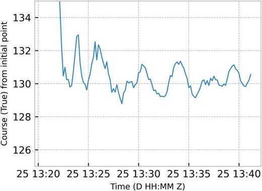
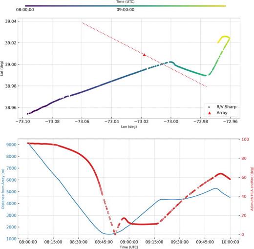
The array was deployed from the R/V Sharp which maneuvered in the vicinity of the array (with and without acoustic augmentation) during the course of the experiment. The global positioning system (GPS) derived heading of the R/V Sharp during the array deployment is shown in Fig. 1. The approximate orientation of the HLA is 131° (true north) corresponding to the heading of the R/V Sharp as it dragged the horizontal leg of the hydrophone array along the bottom before releasing at 1340 Z. In Fig. 2 (top), the GPS track of the R/V Sharp is shown during a two-hour period. The location and estimated orientation of the HLA is also shown in the top panel while the range and orientation of the ship, relative to the array, is shown in the bottom panel of Fig. 2. The orientation of the HLA was confirmed using beamforming during a section of the R/V Sharp track as it approached broadside to the array. This analysis showed array normal to be 42/–138° true north which is consistent the orientation estimated in Fig. 1.

FIG. 1.

(Color online) R/V Sharp GPS course during the last 20 min of the array deployment on JD 238 relative to an initial reference point (at 13:20:40 Z). The ship dragged the HLA along the bottom to straighten the array and released it at 13:40 Z. The approximate course bearing while dragging the array is 131° true north.

FIG. 1.

Close modal

FIG. 2.

(Color online) (Top) R/V Sharp ship track JD 240 0800–1000 Z; approximate array orientation is plotted as a red dashed line. (Bottom) The ship distance from the array (blue) and the approximate azimuth from the array endfire direction (red). The portion of the ship track from 0900 to 0920 Z is approximately 10° off the endfire direction to the HLA.

FIG. 2.

Close modal

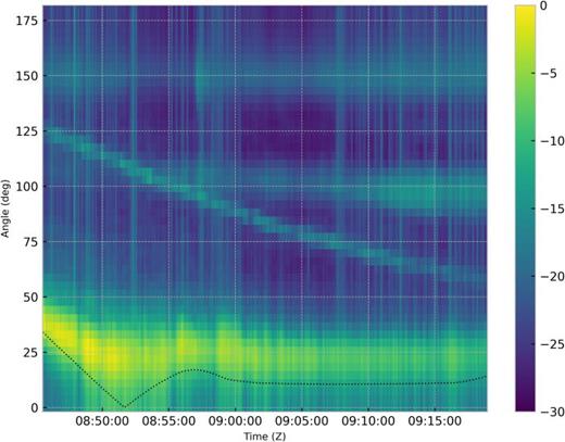
Figure 3 shows the HLA plane wave beamformer output (incoherently averaged over 50–300 Hz) during a segment of the R/V Sharp track as it transited near the array without augmentation. The R/V Sharp passes by and transits approximately endfire to the HLA between 0900 and 0920 Z on Julien Day (JD) 240 as can be seen earlier in Fig. 2 (top). Other unknown ship tracks are also visible in the data. The ground truth azimuth of the R/V Sharp from the endfire direction is shown in Fig. 3 as the red dashed curve. The HLA at endfire measures the conical angle, $ψ$ ⁠, due to the fact that an incoming plane wave with azimuth angle $θ$ and elevation angle $φ$ are related by

FIG. 3.

(Color online) Conventional plane wave beamformer output (incoherently averaged over frequency between 50 and 300 Hz) as R/V Sharp passes by and transits approximately endfire to the HLA between 0900 and 0920 Z on JD 240. Other tracks are also visible in the data. The ground truth azimuth of the R/V Sharp from the endfire direction is shown as the red dashed line (based on GPS).

FIG. 3.

Close modal

The peak in the beamformer output corresponds to this conical angle, $ψ$ ⁠, which is offset from the ship azimuth, $θ$ ⁠, as seen in Fig. 3.

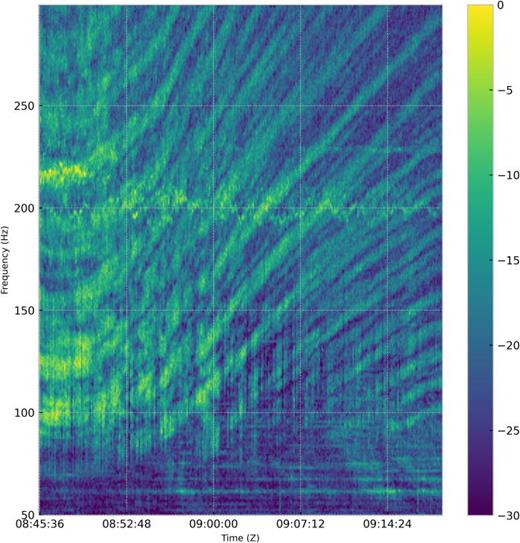
Figure 4 is the single channel power spectrum computed from channel 0 of the HLA for a portion of the JD 240 track shown in Fig. 2. A broadband striation pattern is evident above 90 Hz and there are also spectral lines present in the data. The low frequency acoustic radiation from the R/V Sharp is of interest for wavenumber estimation where the number of modes is limited.

FIG. 4.

(Color online) Power spectrum of HLA Channel 0 as R/V Sharp transits away from the HLA at a near endfire orientation.

FIG. 4.

(Color online) Power spectrum of HLA Channel 0 as R/V Sharp transits away from the HLA at a near endfire orientation.

Close modal

B. Wave number estimation

In the following, multiple methods to estimate the wave numbers on both the horizontal and vertical arrays are compared with simulations based on measured SSP.

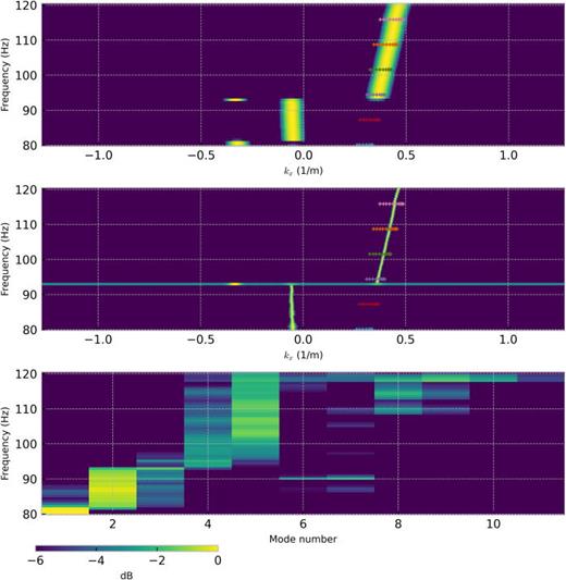
Figure 5 shows processing results obtained using a segment of data from JD 240 from 0900 to 0918 Z. The sampling rate for the data were 11 718.75 samples per second. The spatial separation of the hydrophones was 2.5 m for the vertical and horizontal apertures. The 18-min data segment was transformed to the frequency domain via FFTs of sample length 16 384 points, with 50% overlap, and a Hann window. A singular value decomposition was performed on the l-shaped array (LSA) data. The conventional plane wave beamforming power (top panel) was computed at each frequency with a 512 length zero padded FFT of the HLA component [32 channel component (subvector)] from the leading singular vector. The horizontal wave number axis is corrected for a 10° source azimuth off endfire (i.e., the wave numbers axis is scaled by the factor 1/cos θ_ship, where θ_ship = 10).

FIG. 5.

(Color online) Results from the JD 240 0900–0918 Z track. Top: Conventional beamformer output using the leading eigenvector; x axis is k_x corrected for a 10° source azimuth, y axis is frequency. Above 93 Hz, the leading eigenvector contains significant energy from the azimuth of the R/V Sharp; sources from other azimuths dominate at the lower frequencies. Center: MUSIC beamformer wavenumber estimation with MUSIC with a signal space dimension of 1, x axis is k_x corrected for a 10° source azimuth (off of endfire), y axis is frequency. Bottom: Estimate of modal coefficients using VLA segment of the L-shaped array. Modes 4 and 5 are prominent above 100 Hz. kraken normal mode wavenumbers are computed at six different frequencies using one SSP determined from a temperature profile measured during the same time interval. These modes are overplotted in the top two figures (mode 1 is on the right-hand side). The MUSIC peak is also consistent with the kraken eigenvalues 4 and 5.

FIG. 5.

Close modal

The top panel depicts conventional beamformer output using the leading eigenvector. The x axis is k_x corrected for the 10° source azimuth deviation off endfire. The y axis is frequency. Above 93 Hz, the leading eigenvector contains significant energy from the azimuth of the R/V Sharp; sources from other azimuths dominate at the lower frequencies.

The center panel shows the MUSIC processor power. The signal subspace is assumed to be one-dimensional and given by the leading singular vector, while the noise subspace is spanned by the remaining 31 singular vectors. At each frequency, the noise subspace singular vectors are transformed to the wavenumber domain with a 4096 point zero-padded FFT and incoherently summed. The MUSIC output power is the inverse of the incoherently summed noise subspace power (i.e., it has peaks in the directions of noise subspace power minima).

It is now shown that the dominant measured energy is consistent with modes 4 and 5. The bottom panel shows the modal coefficients using the VLA segment of the L-shaped array. The modal amplitudes are estimated with the VLA data using the eigenvector method [Eq. (9) of Ref. 26] from pressure data. Modes 4 and 5 are prominent above 100 Hz. Representative modal wave numbers computed with the kraken model and corrected for the ship azimuth are plotted on the beamformer and MUSIC outputs.²⁷ One in situ temperature sensor measurements was used to estimate the sound speed profile at the array location and kraken was performed at six different frequencies. The geoacoustic bottom properties for the calculation of the kraken wavenumbers and the simulated data later in Sec. III C are derived from Ref. 28. The geoacoustic model is a 40 m linear gradient layer above a half space derived from previous geoacoustic inversion work in the vicinity. Note, mode 1 is on the right-hand side. Importantly, though the peak of the beamformer output is consistent with the computed wave numbers, the resolution is insufficient for wave number estimation of individual modes. The second panel shows that the MUSIC algorithm (with a signal space of 1) is strongly aligned with mode 4. Unlike the top two panels, the bottom panel is estimated using the vertical segment of the L-shaped array. This also demonstrates that only modes 4 and 5 are prominently detected above 90 Hz.

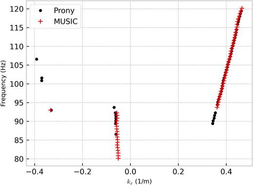
Figure 6 directly compares the wave number estimates from the MUSIC and Prony algorithms. Similar results were obtained, showing a consistency across multiple methods. Note that these methods are able to estimate wavenumbers not only of the desired ship (the R/V Sharp which effectively radiated energy above 90 Hz), but other sources and noise that appear as the wave number estimates near and below k_x = 0.

FIG. 6.

(Color online) Wave number estimation comparison between MUSIC and Prony algorithms.

FIG. 6.

(Color online) Wave number estimation comparison between MUSIC and Prony algorithms.

Close modal

C. Inversion simulation

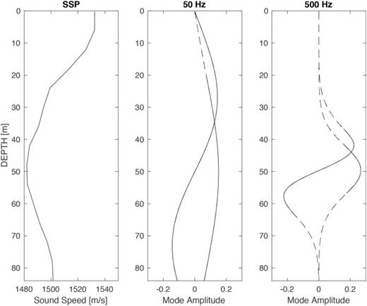
Unique environmental information can be extracted by utilizing wavenumbers over varying modes number or frequency. Figure 7 shows an SSP inferred from conductivity and temperature typical of those measured during LIDDEX. This SSP was used as the unknown for all later inversions. Calculations of the shape and wave numbers of the normal modes was made using KRAKEN. For the purpose of this demonstration, the bottom is treated as a gradient layer over a half-space of known sound speed.²⁹ The first two modes are depicted versus depth at 50 and 500 Hz. It can be seen that the mode shapes are more sensitive to the SSP at higher frequencies such that their vertical extent becomes diminished. Therefore, a diverse set of modes and frequencies interrogates different portions of the water column and increases the uniqueness of the inversion.

FIG. 7.

Calculated normal mode results from a measured SSP is shown at two different frequencies. A diverse set of modes and frequencies interrogates different portions of the water column and increases inversion fidelity (Ref. 14).

FIG. 7.

Close modal

The solid line portion of the modes shows energy trapped between the “turning points.” This corresponds to the transition between oscillating and evanescent energy.²⁹ Individual mode propagation is often associated with its corresponding ray of the same grazing angle and turning points, also known as “ray-mode duality.” At a depth of interest, the grazing angle is defined as $tan θ_{g} (m) = (k_{z} (z)) / k_{m}$ ⁠. Therefore, depending on array placement, not all wavenumbers can be resolved.

In summary, the low frequency modes are useful for providing information throughout the water column, but also interact with the bottom more. Higher frequencies provide stronger information but only in the region in which they are trapped. However, total pressure approaches zero at the surface and is very weak at the bottom interface. Thus, a fundamental limitation of this method is providing information about regions with little to no information (the boundaries and ducts without associated acoustic measurements).

D. Inversions results

In order to highlight the differences between the broadband incoherent L²- and coherent L¹-inversion techniques (recall Sec. II B 3), this section will consider the primary source of error as the starting SSP, while assuming the estimate of the wave numbers to be locally correct. The gross initial guess was a sloped line starting at 1570 m/s and ending at 1450 m/s at the bottom. Three categories of broadband are shown, all starting at 50 Hz, with 50 Hz intervals, reaching 100, 300, or 500 Hz. Even though up to 49 modes were available at 500 Hz, only the first two, at any frequency, were used. The spacing between the first two modes is the largest and thus were predicted to be the easiest to estimate from a realistic hydrophone array while a large number of modes would necessitate very large apertures. L²-inversions were carried out with the well-known pseudoinverse (SVD) which is fast and computationally efficient. L¹-inversions were made using CVX Solver, a fast, robust, and powerful sparse convex optimization tool.³⁰ It is notable that coherent L²- and incoherent L¹-inversion were not shown because the inversions failed or produced inferior results, respectively, within their categories.

Inversion comparisons are displayed in Fig. 8, where the three columns represent the 100, 300, and 500 Hz bandwidths. The top row of panels is the final incoherent L²-solution, and the bottom row of panels is the coherent L¹-inversion solution. The dashed line is the unknown true SSP. All inversions were both solvable and unique. It is clear that increasing the bandwidth improved the results. Amongst the L²-inversions the 500 Hz bandwidth had the lowest mean-squared error (MSE),

FIG. 8.

L²- vs L¹-inversion results for SSP inversion via simulated acoustic wave numbers after 150 and 40 iterations, respectively. The dashed (true) and solid (estimated) SSP is shown for three different bandwidths using only the first two modes. The vertical dashed lines are the physical bounds. The SSP is considered known at the tow depth (“>” at 42 m).

FIG. 8.

Close modal

For all methods, inversion results are weakest near the boundaries. The largest effect that increasing the bandwidth from 300 to 500 Hz had on the L¹-inversions was improving inversion results near the boundaries. However, even with all modes known, the SSP predictions will be biased. Using a better starting estimate of the SSP would decrease the number of iterations necessary for convergence; however, despite a poor starting estimate of the SSP, convergence was achieved.

1. Convergence

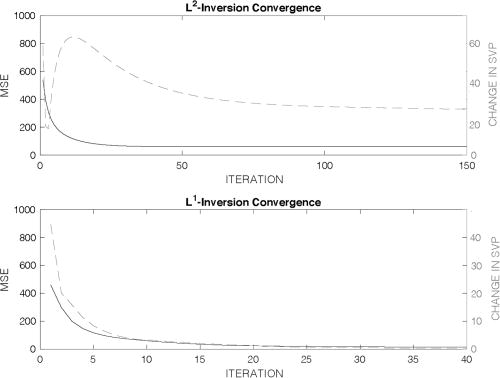
Convergence comparisons between L² and L¹ approaches are shown in Fig. 9. A single L²-inversion is fast but the improvement is slow, thus 150 iterations were necessary. While a single L¹-inversion is slower, only 40 iterations were required. In the end, both methods were computationally similar and near real-time. Mean squared error shows that both methods converge, though the L¹ method converges faster and to lower error. Realistically, the true value of the SSP will not be known. The average of the change in the SSP, from one iteration to the next, can be used as a proxy for convergence.

FIG. 9.

Residual error vs iteration. Mean squared error measurements (solid black) are based on the true SSP. The depth-averaged change in the SSP (dashed gray) can be used as a proxy when using measured data.

FIG. 9.

Close modal

E. Inversion using estimated wave numbers

Section III F shows end-to-end wave number estimation and SSP inversion. The horizontal array aperture of the LIDDEX12 array was small, leading to insufficient spatial resolution for complete determination of all of the wave numbers. Fortunately, due to the close range (starting at ∼2 km) the source level was relatively large. Thus, a large acoustic bandwidth is interrogated, which provides wave number estimates over a large band.

F. Wave number extraction

The horizontal wave numbers estimated over a broad range of frequencies are shown in Fig. 5. Using a sound-speed profile measured in close proximity to the horizontal array, the horizontal wave numbers were simulated using kraken over the same frequencies. The simulated wave numbers have been overlayed as seen in the left side of the figure. Note, these were corrected for the bearing offset from endfire to the array. Due to the limited aperture and number of elements of the horizontal array, only one mode one can be reliably estimated. Note that other sources of energy were present (local and distant shipping); fortunately, these were spatially isolated from the ship-of-opportunity.

The bearing offset was estimated with GPS and beamforming as approximately 10°, respectively. For sake of completeness, the bearing was also estimated by comparing the offset of the estimated and simulated horizontal wave numbers and was found to be ∼ 9.9°.

1. SSP inversion results

In this section, the data-derived estimates of the horizontal wave number will be used to invert for an unknown SSP local to a bottom mounted horizontal array. Within the (array-spacing limited) band up to 300 Hz only one mode was reliably extracted. We will show that this is sufficient information, when combined with other non-acoustic sources, to generally estimate the SSP.

Fixed arrays typically have access to a wide variety of information and processing power. There are many maritime domain awareness products related to weather, ship tracking, oceanography, and other non-acoustic information that are uniquely and reliably available onshore. The use of these sources can help overcome limitations imposed by the limited aperture of the horizontal array used. For the purpose of inversion constraint, knowledge of the sound speed at the depth of the array and the water surface is considered known. A temperature sensor was available at the array, and satellites provided surface temperature. While there are sound speed databases and prediction models that may give a shaped SSP, the starting guess used was a simple line between the extrema.

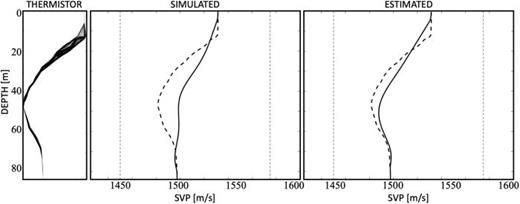
Figure 10 shows the SSP inversion results. The SSP calculated from an array of temperature sensors during the time period of the wave number extraction is shown in the first panel. The set depicts a very common and relatively stable downward refracting shallow water SSP. The singular value decomposition of this set had only one significant value. This indicates that only a sparse amount of information is needed for recovery.

FIG. 10.

SSP inversion results. The first panel shows SSP measurements made over time from a line of temperature sensors. The average SSP over time is shown as a dashed line in the other two panels. The second panel shows the inversion results from horizontal wave numbers simulated from the average SSP. The third panel shows inversions based on wave numbers extracted from the measured data. Note only one mode from 90 to 300 Hz was available for inversion. The vertical dashed lines are the physical bounds. The SSP is considered known at the surface and bottom.

FIG. 10.

Close modal

The mean of the set of SSP is depicted as a dashed line in the last two panels of Fig. 10. This is “notionally” the expected SSP at the convergence of inversion using extracted information. Recall that the ship is moving away from the array from 2 to 4 km over a time frame of about 10 min. Thus, we expect to extract an adiabatic average of horizontal wave numbers. The second panel is an inversion made of kraken generated wave numbers using the dashed profile. The inversion used the first horizontal wave number at five frequencies distributed over the band. The SSP at the top and bottom were constrained. Overall, the inversion quickly and reliably converged to a good approximation of the SSP. Most of the difference between the experimentally estimated SSP and the inverted SSP occurred near the boundary where acoustic information was limited. Additional modes would have improved the fidelity. The final panel shows the inversion results using the data-derived horizontal wave numbers. It qualitatively shows the correct downward refracting profile that was generally present. Like the inversion based on simulated wave numbers, the strength of the duct is probably underrepresented due to the lack of higher order modes. As noted earlier, the starting guess used was a simple line between the extrema.

Additional variations were explored. For instance, using the expected SSP improved convergence rate and stability, but with a similar end result. If the array (and its constraint) had been located in the center of the water column the inversion would better estimate the thermocline at the cost of the sediment interface.

IV. SUMMARY

A methodology to invert for a completely unknown SSP using estimated acoustic wave numbers from a hydrophone array was shown. The iterative inversion is stable, solvable, and unique. It only requires a few modes and is improved by increasing bandwidth. When a large set of wavenumbers over many frequencies is available, inversion via L¹- optimization was shown to be superior. Ultimately, only a limited number of data estimated wave numbers was required to invert for the SSP. Due to the fact that acoustic pressure is reduced near interfaces, this method produces limited results near the surface and bottom. Additionally, in the case of ducts, wave numbers associated with modes trapped in those ducts must be known. Further work is needed to quantify robustness to wave number mismatch and dependence on bottom information.

ACKNOWLEDGMENT

Work supported by the Office of Naval Research.

1. Introduction

Underwater sound is an important carrier of signal propagation in underwater wireless sensor networks. Compared with radio or optical signals, acoustic signals have less attenuation and a better ability to travel over long distances (Erol-Kantarci et al., 2011; Li et al., 2022). Therefore, underwater sound plays an important role in underwater communication, disaster prediction, underwater rescue, sonar ranging, positioning, and other fields (Isik and Akan, 2009; Teymorian et al., 2009; Carroll et al., 2014; Liu et al., 2016; Li et al., 2022; Li et al., 2022). The sound speed profile (SSP) refers to a sets of sound speed values at different depths and at specific latitude and longitude coordinates, which represents a column vector. The traditional methods employed to obtain the SSP consist of direct measurements made using a sound velocity profiler (SVP) or indirect measurements using a conductivity-temperature-depth (CTD) system. However, both SVP and CTD systems usually need to be transported to a designated location by a ship. This process is costly in terms of manpower and time, and the three-dimensional sound speed distribution cannot be quickly obtained.

The development of satellite remote sensing technology allows the continuous observation of sea areas and collection of long-term and large-scale, high-resolution remote sensing data. However, most of the data concerns the ocean surface, and it is difficult to directly monitor ocean depths and investigate important activities occurring in these deeper regions. Nevertheless, most of the deep ocean activities are still related to surface information, and these dynamic phenomena can be analyzed through surface features (Klemas and Yan, 2014). For any given day, the vertical profiles of temperature and salinity from the sea surface to the seafloor can be calculated from regression coefficients (Fox et al., 2002). Then the concept of basis function was proposed to reduce the dimension of the inversion process (Kundu et al., 1975; Tolstoy et al., 1991; Cheng et al., 2022).Carnes proved that there was a functional relationship between remote sensing parameters and empirical orthogonal functions (EOF), and successfully predicted temperature profiles in the northwestern Pacific and northwestern Atlantic Oceans based on this method, which is a single empirical orthogonal function regression(sEOF-r) (Carnes et al., 1990; Carnes et al., 1994). Previous studies had established ocean parameters under a linear framework, but the ocean is a complex nonlinear system, it is difficult to guarantee accuracy in the analysis when describing the ocean parameters with a linear system.

In recent years, machine learning algorithms have been greatly improved (Li et al., 2019; Chen et al., 2020). Bianco et al. provided a detailed overview of the application of machine learning in acoustics and showed that these techniques are very promising in the estimation of ocean parameters, such as seafloor properties, distance, and SSP inversion (Bianco et al., 2019). Among the commonly used machine learning methods with high precision, such as support vector machines, random forests, generalized regression neural networks, ensemble algorithms, etc. The deep learning methods, represented by the recurrent neural network and the convolutional neural network, have achieved good results in the SSP inversion through their powerful model structure. By combining satellite remote sensing data and machine learning, Su et al. and Li et al. used classical machine learning methods and support vector regression to predict global ocean temperature profiles above 1000 m (Su et al., 2015; Li et al., 2017). Li et al. successfully inverted the SSP in the South China Sea through a neural network based on a self-organizing map (Li et al., 2021).

In the present study, the South China Sea was selected as the inversion area. The region is affected by the monsoon season and the complex terrain of the seabed, frequent marine activities, eddies, internal solitary waves and other dynamics, therefore it is difficult to invert the profile. Due to the influence of various factors, the South China Sea has obvious regional and seasonal characteristics, and especially in the summer, the strong sunshine forms a large negative temperature gradient. The aim of this study was to propose a method for reconstructing the SSP based on an extensible end-to-end tree boosting (XGBoost) model (Chen and Guestrin, 2016). The method was applied to invert the SSP of the South China Sea (above 1000 meters) in different seasons in 2018. In addition, the accuracy of the model was estimated and its robustness and stability were evaluated with respect to seasons.

2. Materials and methods

2.1. EOF dimensionality reduction

The SSP can be calculated using the sound speed empirical formula, combined with water temperature and salinity. The temperature profile can be inverted by sea surface parameters, and it has a relatively stable temperature–salinity relationship with the salinity profile. Therefore, the SSP can be obtained by inversion based on the sea surface parameters. On this basis, LeBlanc proposed that the EOF was the minimum basis function for inverting the SSP, which can be expressed as (Leblanc and Middleton, 1980):

$\begin{array}{l} C (z) = C_{0} (z) + \sum_{s = 1}^{\infty} α_{s} k_{s} (z) & (1) \end{array}$

Where C(z) is a column vector, representing the sound speed distribution at a particular latitude and longitude, and the elements of the vector represent the sound speed values at different depths. C₀(z) is the long-term, stable background profile of the ocean, usually calculated as an average of many years, K_S(z) is the EOF, and α_s is the EOF’s projection coefficient, its subscript s is the modal number of the EOF. Generally, the higher the order, the greater the background noise. Considering the reconstruction accuracy and noise suppression combined with the previous research on profile reconstruction, the fifth-order EOF mode is here selected to reconstruct the SSP. The EOF is the most commonly used perturbation shape function in SSP inversion and is the main mode capable of identifying ocean perturbations (Pauthenet et al., 2017). The EOF modes can be obtained by extracting the principal components of the SSP sample matrix. The SSP anomaly matrix Y is an n×m matrix, where n refers to n discrete depths per section and m refers to the total number of sections, and it is calculated by subtracting the background profile from each SSP sample matrix. The EOF modes of various of orders can be derived from principal component analysis as follows (Kundu et al., 1975):

Where X is the covariance matrix of Y The eigenvalue is λ. k is the modal function of each order of EOF. In this study, the fifth-order EOF modal function is used to invert the SSP. In order to adapt the model to noise generated by background profile, a sequence of all 1s is artificially added before the fifth-order EOF mode as the 0-order mode. By regressing k and Y the projection coefficient (α_0,α₁,α₂,α₃,α₄,α₅) Is obtained and the SSP can be expressed as:

$\begin{array}{l} C (z) = C_{0} (z) + α_{0} k_{0} (z) + α_{1} k_{1} (z) + α_{2} k_{2} (z) + α_{3} k_{3} (z) + α_{4} k_{4} (z) + α_{5} k_{5} (z) & (4) \end{array}$

2.2. Profile estimation based on remote sensing data

2.2.1. Inversion based on sEOF-r

With the development of remote sensing technology, a large amount of data has been continuously accumulated, providing a stable basis for the statistics of linear regression. Based on the regression analysis of a large number of samples, the observed sea surface height anomaly (SSHA), sea surface temperature anomaly (SSTA), and EOF projection coefficient A can be approximated as a linear relationship. Using this approximate linear relationship for the linear fitting (Chen et al., 2018), the following relationship is obtained:

$\begin{array}{l} \begin{array}{l} α_{i} (t) = A_{i, 0} + A_{i, 1} \times S S H A (t) + A_{i, 2} \times S S T A (t) + A_{i, 3} \times S S H A (t) \times S S T A (t) \\ , i = 0, 1, 2, 3, 4, 5 \end{array} & (5) \end{array}$

where A_i is the coefficient obtained by linear fitting and i represents the EOF order. The SSHA and SSTA of the test data are input into Equation (5) to calculate the projection coefficient A_{i ,}and then this is substituted into Equation (4) to invert the SSP. Obviously, the sEOF-r model is obtained by linear fitting based on a large number of samples. This linear relationship is a statistical result, and samples with large differences between individual and statistical characteristics are often difficult to handle (Stammer, 1997; Wunsch, 1997).

2.2.2. Inversion based on the XGBoost model

Considering that samples with large differences between individual and statistical characteristics will cause large errors and that the ocean is a complex dynamic system. It is believed that the accuracy of inversion can be improved by breaking the constraints of linear inversion. To this end, we introduce a scalable end-to-end tree boosting model called XGBoost. The objective function of this model is written as a traditional loss function plus the model complexity, as follows:

$\begin{array}{l} O b j = \sum_{i = 1}^{m} l (y_{i}, \hat{y_{i}}) + \sum_{i = 1}^{K} Ω (f_{k}) & (6) \end{array}$

Where i represents the i-th sample, m represents the total amount of data imported into the k-th tree, and K represents all the trees established by the model. y_i is the true value and $\hat{y_{i}}$ is the predicted value. After calculation, the formula can be transformed into:

$\begin{array}{l} \begin{array}{l} O b j = \sum_{i = 1}^{m} [l (y_{i}^{t}, {\hat{y}}_{i}^{(t - 1)}) + f_{t} (x_{i}) g_{i} + \frac{1}{2} {(f_{t} (x_{i}))}^{2} h_{i}] + \sum_{i = 1}^{t - 1} Ω (f_{k}) + Ω (f_{t}) \\ = \sum_{i = 1}^{m} [f_{t} (x_{i}) g_{i} + \frac{1}{2} {(f_{t} (x_{i}))}^{2} h_{i}] + Ω (f_{t}) \end{array} & (7) \end{array}$

where t represents the t-th iteration, g_i and h_i are the first and second derivatives of ${\hat{y}}_{i}^{(t - 1)}$ on $l (y_{i}^{t}, {\hat{y}}_{i}^{(t - 1)})$ , respectively. XGBoost is a natural overfitting model, so a regular term needs to be introduced to penalize it. In this study, the regular terms L1 and L2 are introduced in the following equation:

$\begin{array}{l} \begin{array}{l} Ω (f_{t}) = Υ T + \frac{1}{2} α \sum_{j = 1}^{T} | ω_{j} | + \frac{1}{2} λ \sum_{j = 1}^{T} ω_{j}^{2} \end{array} & (8) \end{array}$

where T represents the total number of leaf nodes, j is the index of each leaf node, $ω_{j}$ is the sample weight on the leaf node, and Y is a certain tree.

Then, q(x_i) is used to represent the leaf node where sample x_i is located, and $ω_{q (x_{i})}$ $ω_{j}$ to represent the score obtained by the sample falling to the q(x_i)-th leaf node on the k-th tree, which results in the following equation:

Equations (8) and (9) are substituted into equation (7) to obtain:

$\begin{array}{l} O b j = \sum_{i = 1}^{m} [ω_{q (x_{i})} g_{i} + \frac{1}{2} ω_{q (x_{i})}^{2} h_{i}] + Υ T + \frac{1}{2} α \sum_{j = 1}^{T} | ω_{j} | + \frac{1}{2} λ \sum_{j = 1}^{T} ω_{j}^{2} & (10) \end{array}$

The $ω_{j}$ on each leaf is the same. The difference is the g_i corresponding to each sample, therefore all samples have to be assigned to any node of the T leaf node clock. Consequently, the set of samples contained in the leaf with index j is defined as I_j. Given that $G_{j} = \sum_{i \in I_{j}} g_{i}$ , $H_{j} = \sum_{i \in I_{j}} h_{i}$ , equation (10) could be transformed into:

$\begin{array}{l} \begin{array}{l} O b j = \sum_{j = 1}^{T} \begin{matrix} (ω_{j} \times \sum_{i \in I_{j}} g_{i}) + \frac{1}{2} \sum_{j = 1}^{T} (ω_{\begin{array}{l} j \end{array}}^{2} \times \sum_{i \in I_{j}} h_{i}) + Υ T + \frac{1}{2} α \sum_{j = 1}^{T} | ω_{j} | + \frac{1}{2} λ \sum_{j = 1}^{T} ω_{j}^{2} \end{matrix} \\ = \sum_{j = 1}^{T} [ω_{j} G_{j} + \frac{1}{2} ω_{j}^{2} (H_{j} + λ + α)] + Υ T \end{array} & (11) \end{array}$

Given that $F^{*} (ω_{j}) = ω_{j} G_{j} + \frac{1}{2} ω_{j}^{2} (H_{j} + λ + α)$ (12)

the objective function is the minimum when $F^{*} (ω_{j})$ takes the minimum value. Therefore, the derivative of $ω_{j}$ is obtained from $F^{*} (ω_{j})$ , and the extreme value of the objective function is obtained when the first derivative is equal to 0, which in this case resulted in:

Then, equation (13) is substituted into equation (11) to obtain:

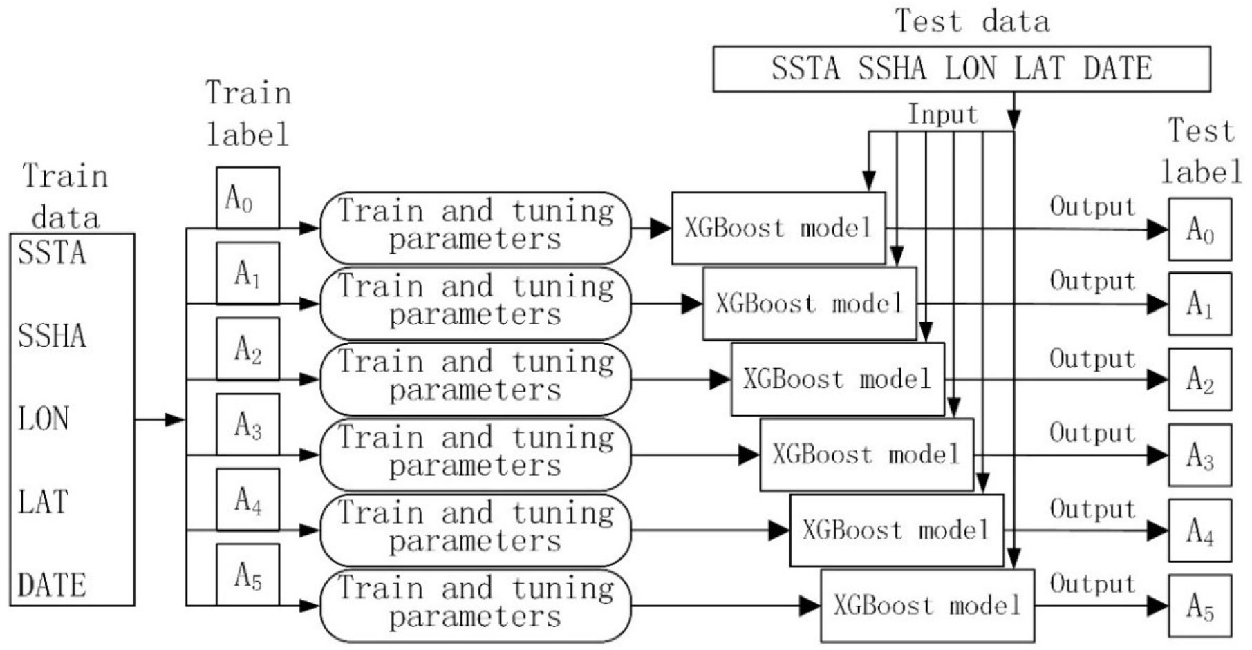
$\begin{array}{l} O b j = - \frac{1}{2} \sum_{j = 1}^{T} \frac{G_{j}^{2}}{H_{j} + λ + α} + Υ T & (14) \end{array}$

Equation (14) shows that λ, α, and Y are the set hyperparameters, Gj and H_j Are jointly determined by the loss function and the prediction result under this structure, and T is only determined by the tree structure. Therefore, the objective function is a function of T. The effect of the model is directly related to the total number of leaf nodes and the structure of the tree, the smaller the objective function, the better the structure of the tree. This is the advantage of the XGBoost model. Figure 1 shows the XGBoost model training and testing process. Firstly, a dataset was created including all the data from 2009 to 2018, such as the remote sensing parameters SSHA and SSTA, LAT and LON, DATE. LAT and LON are obtained by taking the cosine of latitude and longitude, and DATE is obtained by ordering the measurement time of the sample. Secondly, according to the year, the 2009–2017 data were assigned to the training data, and the 2018 data were assigned to the test data. Third, the projection coefficient was used as the model output label, and the coefficients for the 2009–2017 period and those for 2018 were divided into training labels and test labels, respectively. Because the XGBoost model was a single-output regression model, it was necessary to regress the coefficients of each order separately. Then, the SSP was inverted based on equation (4), and the accuracy of the model was evaluated by the root mean square error (RMSE).

Figure 1 Flow chart of the XGBoost model training and testing.

3. Data

3.1. Satellite remote sensing data

The study used sea surface height data and sea surface temperature data from the 2009–2018 period, which were obtained from the AVISO data center and from daily data sourced at NOAA data centers in the United States, respectively. The time resolution of the above two datasets was 1 day and their spatial resolution was 0.25° × 0.25°.

3.2. Background profile data

The background profile is the constant part in the SSP reconstruction. The background profile comprised climate profile data obtained from the World Ocean Atlas (WOA13) (https://www.nodc.noaa.gov/0C5/woal3/) and it contained the average values of temperature, salinity, and other parameters. This study selected the data of WOA13 in the South China Sea, with a spatial resolution of 1°×1°, were selected.

3.3. Argo data

The Argo data were obtained from the “Global Ocean Argo Scatter Dataset” (ftp://ftp.argo.org.cn/pub/ARGO/global/). All the temperature and salinity profiles measured in the South China Sea from 2009 to 2018 were selected, and the sound speed empirical formula was used to convert the data into the SSP. Interpolate the SSP to the same sampling rate as the background profile.

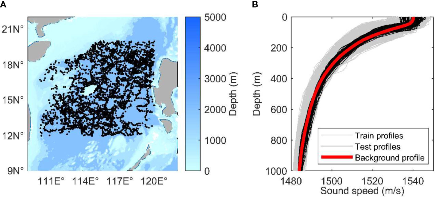
The areas covering the 12°–20°N and 110°–120°E coordinates in the South China Sea were selected as the inversion regions. The study area has a complex topography, a monsoon climate, and frequent marine activities, such as eddies and internal solitary waves. The combination of these factors challenges the validity of the model. Figure 2A shows the distribution of all samples, amounting to a total of 3881 SSPs. Figure 2B shows the divided training and test data. The profiles from 2009 to 2017 were divided into training data for a total of 3757 items, while the profiles of year 2018 were divided into test data for a total of 124 items.

Figure 2 (A) Distribution of the Argo samples in the South China Sea. (B) Training, test, and background profiles.

3.4. EOF analysis

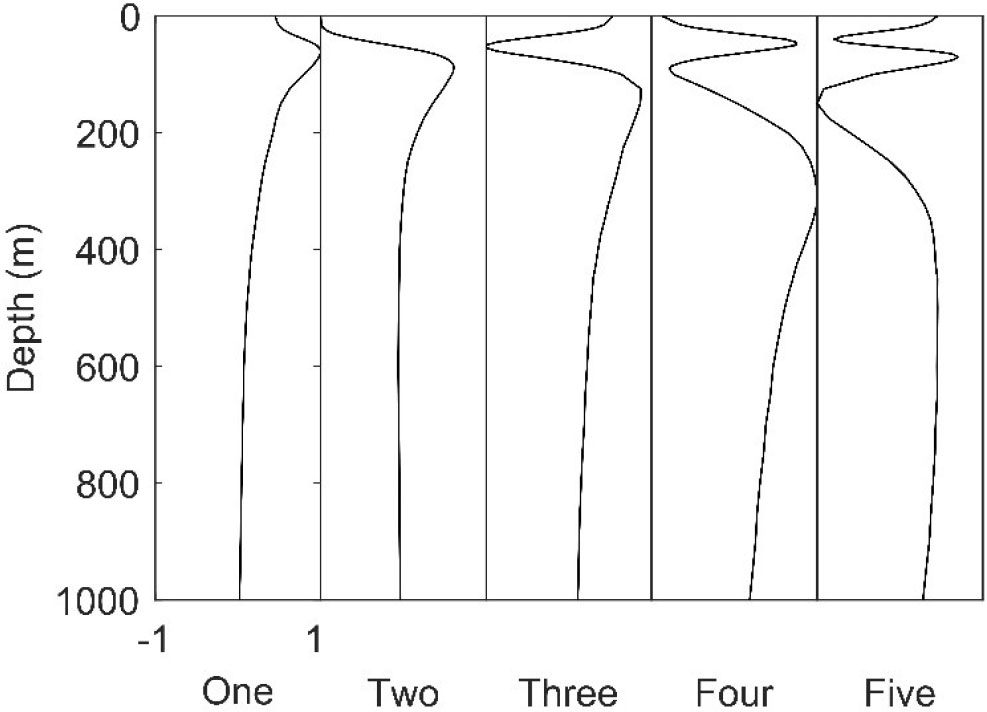
The EOF can describe the perturbation of most SSP features and reduce the dimension of the perturbation of a sample (Carnes et al., 1994). Figure 3 shows the first five modes after EOF normalization, excluding the zero-order mode. From the perspective of the EOF amplitude distribution, the perturbation mainly occurred at a depth of about 100 m, and the perturbation was close to zero at about 1000 m. The samples in the South China Sea are sparse, and the larger the depth, the fewer the samples. Considering the number of samples and EOF perturbation, the research focuses on SSP inversion within 1000 meters.

Figure 3 The first five modes of normalized EOF.

Table 1 presents the reconstruction properties of the 1st-to-5th-order EOFs. The contribution rates of these five EOF modes to the variance were 70.72%, 16.24%, 4.67%, 3.30%, and 1.57%, respectively, and the cumulative variance contribution was 96.50%. Although the inversion range was large, there were still several major EOF modes that could describe most of the changes, which confirmed the consistency of the EOF in the South China Sea. The average reconstruction error of the 5th-order EOF was 0.60 m/s, indicating that the reconstruction of this EOF was accurate. Therefore, in the subsequent comparison of the sEOF-r model with the XGBoost model, the SSP was reconstructed using the 5th-order EOF.

Table 1 Variance contribution rate and error of the 1st-to-5th-order EOFs reconstruction.

4. Results and discussion

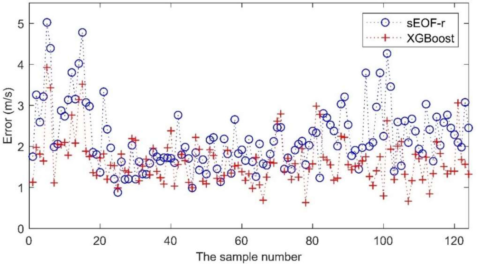
In this study, the RMSE was used as the precision evaluation index to assess the effect of the two models in the profile inversion in the South China Sea. For the SSP, the RMSE of the XGBoost inversion was 1.75 m/s, and that of the sEOF-r inversion was 2.34 m/s, and the reconstruction accuracy was improved by 25%. Figure 4 shows the error comparison between the sEOF-r and XGBoost models during SSP reconstruction. Except for individual samples, the inversion accuracy of the XGBoost model was significantly better than that of the sEOF-r model. The maximum and average SSP inversion errors produced in the sEOF-r model were 5.02 and 2.21 m/s, respectively, while those produced in the XGBoost model were 3.92 and 1.66 m/s, also respectively. In addition, most of the inversion errors of the XGBoost model were below 1.70 m/s, and their total variance was 0.33 m/s, which was much lower than the value of 0.62 m/s measured in the sEOF-r model. The qualities of robustness and stability were better in the XGBoost than in the sEOF-r model. The latter was obtained by linear fitting based on a large number of samples. This linear relationship represented a statistical result, and it was difficult to deal with samples with large differences between individual and statistical characteristics (Stammer, 1997; Wunsch, 1997). Therefore, the ensemble XGBoost learning algorithm was introduced to eliminate the constraints of linear inversion. In this algorithm, latitude, longitude parameters and time parameters of measuring were introduced to improve the inversion accuracy Especially in samples with large errors, the effect was significant. For example, the maximum error of the XGBoost model inversion was 1.10 m/s smaller than that of the sEOF-r model, and the maximum error of the two models happened to be generated in the same sample. The results showed that the XGBoost model was more suitable than the linear sEOF-r model for defining the complex marine activities of the South China Sea.

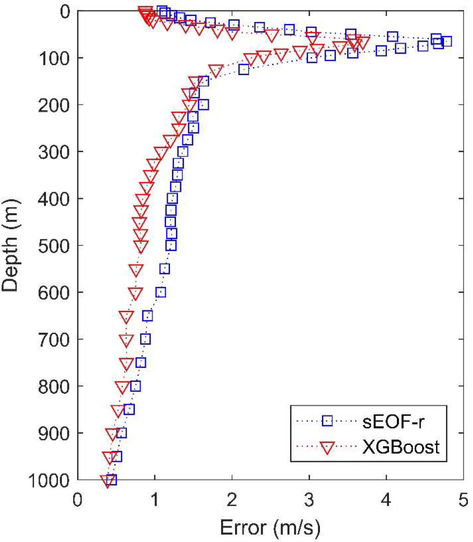
Figure 4 Reconstruction error of two models for different samples.

Figure 5 shows the reconstruction error at different depths. At all depths, the XGBoost model produced smaller errors than the sEOF-r model. For both models, the maximum error was generated at depths close to 100 m, with values of 4.78 m/s for the sEOF-r model and 3.69 m/s for the XGBoost model, which was consistent with the perturbation range of the leading mode in Figure 3. Temperature is the main factor influencing the variation of the speed of sound. Therefore, the sea surface parameters have great influence on the calculation of sea surface sound speed, so the error is small. with large seasonal and diurnal variations in the temperature of the mixed layer, as well as internal solitary waves and other oceanic dynamic activities, leading to the concentration of errors at these depths. When the depth exceeds the mixing layer, the error becomes smaller because the disturbance of the basis function becomes smaller.

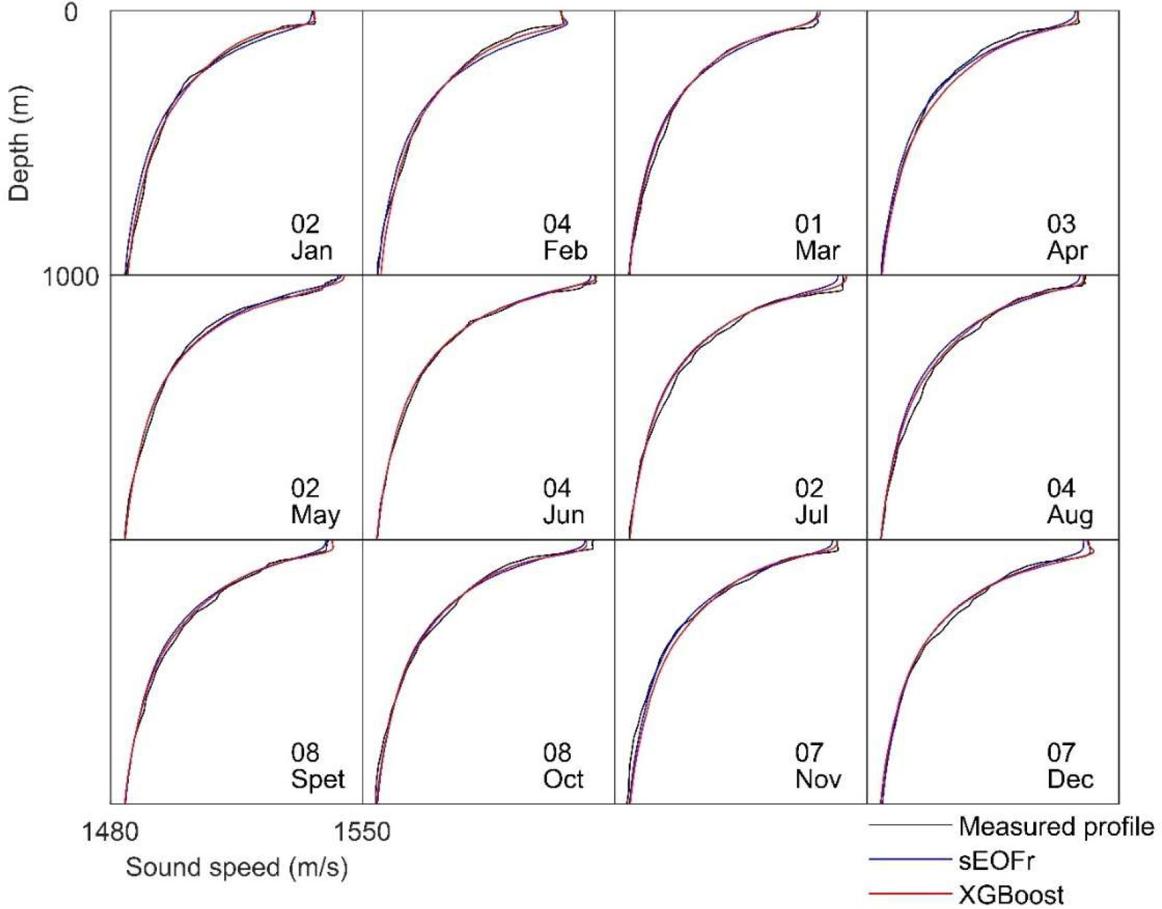
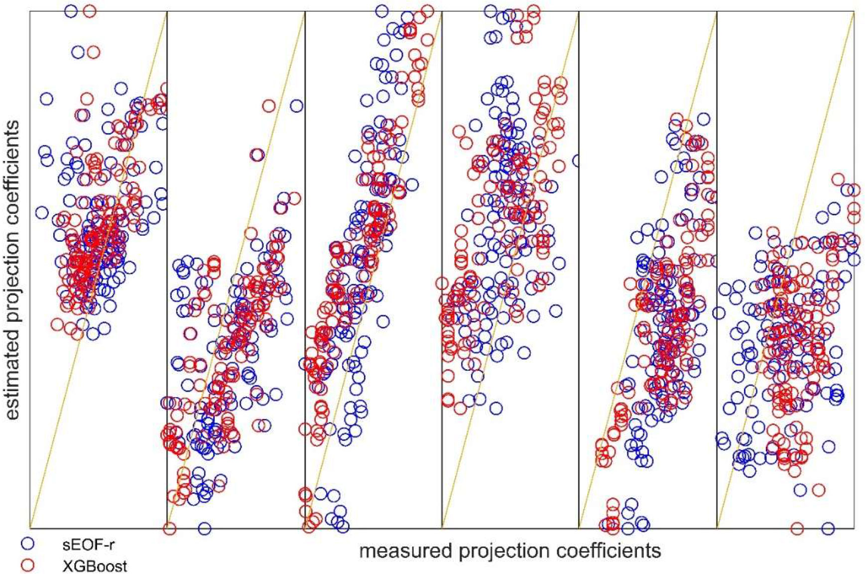
Figure 5 Reconstruction errors of the sEOF-r and XGBoost models at different depths.

Figure 6 shows the first SSP of each month in the reconstructed SSP. The results were consistent with those reported in Figures 4, 5, showing that XGBoost is closer to the measurement profile than the sEOF-r model in almost every sample. This also indicates that the linear model will produce large errors when dealing with numerous samples, especially if containing large differences between individual and statistical characteristics. In the XGBoost model, the simple linear law was broken, and the resulting error was small. Figure 7 shows a comparison of the measured and estimated values of the 0-to-5th-order projection coefficients. Clearly, the ensemble learning model provided better results, and the linear sEOF-r model lagged behind in most cases. As the order increased, the error of the projection coefficient tended to increase. In general, the higher the order, the greater the background noise. Considering the reconstruction accuracy and noise suppression, it is concluded that choosing the 5th-order EOF inversion is sufficient to ensure reconstruction accuracy.

Figure 6 Reconstruction results of the first effective profile for each month.

Figure 7 Results of the inversion of the normalized projection coefficients of the first five orders. The straight line indicates perfect inversion. The five orders, from zero to the fifth, are indicated from left to right.

5. Conclusions

The present study proposed a method for reconstructing the SSP based on XGBoost model using SSHA, SSTA, LAT, LON, and DATE as the input data, and the 0-to-5th-order projection coefficients as the output data. Both input and output data were then converted into training data for the 2009–2017 period and test data for 2018 years. The XGBoost model was trained through the training data, and then the test data was used to obtain the SSP’s projection coefficient in 2018. Based on this, the 2018 SSP was inverted, and the RMSE was used as the evaluation metric of the model’s accuracy. The results showed that the RMSE of the XGBoost model was 1.75 m/s, which was 25% less than the 2.34 m/s error detected in the sEOF-r model. Compared with the linear regression model, the XGBoost model showed a better performance. Specifically, it overcame linear constraints, more relevant parameters could be introduced for regression (such as longitude and latitude, measurement date, etc.), there was no analytical restriction, and the relationship between parameters could be more easily discovered. The experiments showed that the XGBoost model had a better and more robust effect than the linear model in the inversion of SSP information.

Data availability statement

The original contributions presented in the study are included in the article/supplementary material. Further inquiries can be directed to the corresponding author.

Author contributions

ZO completed the literature research, analysis, and manuscript writing. KQ completed the Conceptualization, methodology and funding acquisition. MS, YW, and JZ jointly completed the validation, visualization and project administration. All authors contributed to the article and approved the submitted version.

Funding

This research was funded by the Natural Science Foundation of Guangdong Province, grant number No.2022A1515011519.

Conflict of interest

The authors declare that the research was conducted in the absence of any commercial or financial relationships that could be construed as a potential conflict of interest.

Publisher’s note

All claims expressed in this article are solely those of the authors and do not necessarily represent those of their affiliated organizations, or those of the publisher, the editors and the reviewers. Any product that may be evaluated in this article, or claim that may be made by its manufacturer, is not guaranteed or endorsed by the publisher.

References

Bianco M. J., Gerstoft P., Traer J., Ozanich E., Roch M. A., Gannot S., et al. (2019). Machine learning in acoustics: Theory and applications. J. Acoust. Soc Am. 146, 3590–3628. doi: 10.1121/1.5133944

PubMed Abstract | CrossRef Full Text | Google Scholar

Carnes M. R., Mitchell L., Dewitt P. W. (1990). Synthetic temperature profiles derived from GEOSAT altimetry : comparison with air-dropped expendable bathythermograph profiles. J. Geophys. Res. Atmos. 95, 17979–17992. doi: 10.1029/JC095iC10p17979

CrossRef Full Text | Google Scholar

Carnes M. R., Teague W. J., Mitchell J. L. (1994). Inference of subsurface thermohaline structure from fields measurable by satellite. J. Atmos. Ocean. Technol. 11, 551–566. doi: 10.1175/1520-0426(1994)011<0551

CrossRef Full Text | Google Scholar

Carroll P., Mahmood K., Zhou S., Zhou H., Xu X., Cui J.-H. (2014). On-demand asynchronous localization for underwater sensor networks. IEEE Trans. Signal Process. 62, 3337–3348. doi: 10.1109/TSP.2014.2326996

CrossRef Full Text | Google Scholar

Cheng L., Ji X., Zhao H., Li J., Xu W., et al. (2022). Tensor-based basis function learning for three-dimensional sound speed fields. J. Acoustical Soc. America 151, 269. doi: 10.1121/10.0009280

CrossRef Full Text | Google Scholar

Chen C., Ma Y., Liu Y. (2018). Reconstructing sound speed profiles worldwide with sea surface data. Appl. Ocean Res. 77, 26–33. doi: 10.1016/j.apor.2018.05.002

CrossRef Full Text | Google Scholar

Chen C., Yan F., Gao Y. A., Jin T., Zhou Z. (2020). Improving reconstruction of sound speed profiles using a self-organizing map method with multi-source observations. Remote Sens. Lett. 11:6, 572–580. doi: 10.1080/2150704X.2020.1742940

CrossRef Full Text | Google Scholar

Erol-Kantarci M., Mouftah H. T., Oktug S. (2011). A survey of architectures and localization techniques for underwater acoustic sensor networks. IEEE Commun. Surv. Tut. 13, 487–502. doi: 10.1109/SURV.2011.020211.00035

CrossRef Full Text | Google Scholar

Fox D. N., Teague W. J., Barron C. N., Carnes M. R., Lee C. M. (2002). The modular ocean data assimilation system (MODAS). J. Atmos. Ocean. Technol. 19, 240–252. doi: 10.1175/1520-0426(2002)019<0240

CrossRef Full Text | Google Scholar

Isik M. T., Akan O. B. (2009). A three dimensional localization algorithm for underwater acoustic sensor networks. IEEE Trans. Wirel. Commun. 8, 4457–4463. doi: 10.1109/TWC.2009.081628

CrossRef Full Text | Google Scholar

Klemas V., Yan X. H. (2014). Subsurface and deeper ocean remote sensing from satellites: An overview and new results. Prog. Oceanogr. 122, 1–9. doi: 10.1016/j.pocean.2013.11.010

CrossRef Full Text | Google Scholar

Kundu P. K., Allen J. S., Smith R. L. (1975). Modal decomposition of thevelocity field near the Oregon coast. J.Phys.Oceanogr. 5, 683–704. doi: 10.1175/1520-0485(1975)005<0683:MDOTVF>2.0.CO;2

CrossRef Full Text | Google Scholar

Leblanc L. R., Middleton F. H. (1980). An underwater acoustic sound velocity data model. J. Acoust. Soc Am. 67, 2055–2062. doi: 10.1121/1.384448

CrossRef Full Text | Google Scholar

Li Y., Gao P., Tang B., Yi Y., Zhang J. (2022). Double feature extraction method of ship-radiated noise signal based on slope entropy and permutation entropy. Entropy 24, 22. doi: 10.3390/e24010022

CrossRef Full Text | Google Scholar

Li Y., Geng B., Jiao S. (2022). Dispersion entropy-based lempel-ziv complexity: A new metric for signal analysis. Chaos Solitons Fractals. 161, 112400. doi: 10.1016/j.chaos.2022.112400

CrossRef Full Text | Google Scholar

Li H., Qu K., Zhou J. (2021). Reconstructing sound speed profile from remote sensing data: Nonlinear inversion based on self-organizing map. IEEE Access 9, 109754–109762. doi: 10.1109/ACCESS.2021.3102608

CrossRef Full Text | Google Scholar

Li Q., Shi J., Li Z., Luo Y., Yang F., Zhang K., et al. (2019). Acoustic sound speed profile inversion based on orthogonal matching pursuit. Acta Oceanol. Sin. 38, 149–157. doi: 10.1007/s13131-019-1505-4

CrossRef Full Text | Google Scholar

Li W., Su H., Wang X., Yan X. H. (2017). Estimation of global subsurface temperature anomaly based on multisource satellite observations. J. Remote. Sens. 21, 881–891. doi: 10.11834/jrs.20177026

CrossRef Full Text | Google Scholar

Li Y., Tang B., Yi Y. (2022). A novel complexity-based mode feature representation for feature extraction of ship-radiated noise using VMD and slope entropy. Appl. Acoustics. 196, 108899. doi: 10.1016/j.apacoust.2022.108899

CrossRef Full Text | Google Scholar

Liu J., Wang Z., Cui J.-H., Zhou S., Yang B. (2016). A joint time synchronization and localization design for mobile underwater sensor networks. IEEE Trans. Mob. Comput. 15, 530–543. doi: 10.1109/TMC.2015.2410777

CrossRef Full Text | Google Scholar

Pauthenet E., Roquet F., Madec G., Nerini D. (2017). A linear decomposition of the southern ocean thermohaline structure. J. Phys. Oceanogr. 47, 27–47. doi: 10.1175/JPO-D-16-0083.1

CrossRef Full Text | Google Scholar

Stammer D. (1997). Global characteristics of ocean variability estimated from regional TOPEX/POSEIDON altimeter measurements. J. Phys. Oceanogr. 27, 1743–1769. doi: 10.1175/1520-0485(1997)027<1743

CrossRef Full Text | Google Scholar

Su H., Wu X., Yan X. H., Kidwell A. (2015). Estimation of subsurface temperature anomaly in the Indian ocean during recent global surface warming hiatus from satellite measurements: A support vector machine approach. Remote Sens. Environ. 160, 63–71. doi: 10.1016/j.rse.2015.01.001

CrossRef Full Text | Google Scholar

Teymorian A. Y., Cheng W., Ma L., Cheng X., Lu X., Lu Z. (2009). 3D underwater sensor network localization. IEEE Trans. Mob. Comput. 8, 1610–1621. doi: 10.1109/TMC.2009.80

CrossRef Full Text | Google Scholar

Tolstoy A., Diachok O., Frazer L. N. (1991). Acoustic tomography via matched field processing. J.Acoust. Soc.Am. 89, 1119–1127. doi: 10.1121/1.400647

CrossRef Full Text | Google Scholar

Wunsch C. (1997). The vertical partition of oceanic horizontal kinetic energy. J. Phys. Oceanogr. 27, 1770–1794. doi: 10.1175/1520-0485(1997)027<1770

CrossRef Full Text | Google Scholar

Sunday, February 25, 2024

Through the sensor estimation of sound speed profiles | The Journal of the Acoustical Society of America | AIP Publishing

I. INTRODUCTION

II. THEORY

A. Wave number estimation

1. Normal mode representation

2. Covariance matrix

3. Plane wave beamforming

4. MUSIC algorithm

5. Prony algorithm

B. Sound speed profile inversion

1. Problem formalization

2. Solvability and uniqueness

3. Utilizing mode and frequency observation diversity

III. SIMULATION AND EXPERIMENT

A. LIDDEX12

B. Wave number estimation

C. Inversion simulation

D. Inversions results

1. Convergence

E. Inversion using estimated wave numbers

F. Wave number extraction

1. SSP inversion results

IV. SUMMARY

ACKNOWLEDGMENT

Estimation of sound speed profiles based on remote sensing parameters using a scalable end-to-end tree boosting model

1. Introduction

2. Materials and methods

2.1. EOF dimensionality reduction

2.2. Profile estimation based on remote sensing data

2.2.1. Inversion based on sEOF-r

2.2.2. Inversion based on the XGBoost model

3. Data

3.1. Satellite remote sensing data

3.2. Background profile data

3.3. Argo data

3.4. EOF analysis

4. Results and discussion

5. Conclusions

Data availability statement

Author contributions

Funding

Conflict of interest

Publisher’s note

References

No comments:

Post a Comment

Breakthrough in Satellite Error Correction Improves Space Communications