Deep operator learning-based surrogate models for aerothermodynamic analysis of AEDC hypersonic waverider

A schematic representation of a DeepONet that is trained to learn the mapping from the input function $f$ to the output function $𝒢(f)(y)$, evaluated at $y$. DeepOnet consists of a branch and a trunk network.

Deep operator learning-based surrogate models for aerothermodynamic analysis of AEDC hypersonic waverider

Physics > Fluid Dynamics

[Submitted on 21 May 2024]

Khemraj Shukla, Jasmine Ratchford, Luis Bravo, Vivek Oommen, Nicholas Plewacki, Anindya Ghoshal, George Karniadakis

Comments:	71st JANNAF Propulsion Meeting, Oklahoma City, OK, 6-10 May 2024, 10 pages, 6 figures
Subjects:	Fluid Dynamics (physics.flu-dyn)
Cite as:	arXiv:2405.13234 [physics.flu-dyn]
	(or arXiv:2405.13234v1 [physics.flu-dyn] for this version)
	https://doi.org/10.48550/arXiv.2405.13234

Submission history

From: Jasmine Ratchford [view email]
[v1] Tue, 21 May 2024 22:40:59 UTC (10,109 KB)

 Summary

This research paper explores the use of deep operator learning-based surrogate models, specifically DeepONets, for aerothermodynamic analysis of hypersonic vehicles. The key points are:

1. DeepONets are neural networks that can approximate operators, learning function-to-function mappings, making them suitable for creating surrogate models for computationally expensive hypersonic aerothermodynamic models.

2. The authors investigated the use of DeepONets to infer flow fields (volume and surface quantities) around a 3D waverider model based on experimental data from the Arnold Engineering Development Center (AEDC) Hypervelocity Wind Tunnel.

3. They employed a two-step training approach for the DeepONets to accurately approximate solutions in the presence of discontinuities caused by shocks across the entire volume.

4. DeepONet models were trained to predict pressure, density, velocity, heat flux, and total shear stress for the AEDC waverider geometry at various angles of attack.

5. The trained DeepONets effectively captured shock locations and demonstrated minimal generalization error, enabling accurate flow field predictions with a significant speed-up compared to traditional CFD solvers.

The authors conclude that DeepONets are versatile and capable of handling complex issues in high-speed flow regimes, making them suitable for various engineering applications, including shape optimization. The framework presented can be extended to accommodate adaptive geometry and optimization in unsteady flows with shocks and non-equilibrium chemistry. 

DeepONets

Short for Deep Operator Networks, are a type of neural network architecture designed to learn nonlinear operators between function spaces. They were introduced by Lu et al. in 2019 and are based on the universal approximation theorem for operators.

Key aspects of DeepONets:

1. Architecture: A DeepONet consists of two sub-networks: a branch network and a trunk network. The branch network encodes the input function, while the trunk network learns a set of basis functions. The final output is obtained by computing the inner product between the outputs of the branch and trunk networks.
2. Function-to-function mappings: Unlike traditional neural networks that learn mappings between finite-dimensional spaces, DeepONets learn mappings between infinite-dimensional function spaces. This allows them to approximate complex nonlinear operators, such as those arising from partial differential equations (PDEs).
3. Universality: DeepONets are universal approximators for nonlinear operators, meaning they can theoretically approximate any continuous nonlinear operator to arbitrary accuracy, given sufficient network depth and width.
4. Applications: DeepONets have been applied to various problems, including learning solution operators of PDEs, modeling dynamic systems, and creating surrogate models for computationally expensive simulations. They have shown promise in fields such as fluid dynamics, material science, and engineering design optimization.
5. Variants and extensions: Several variants and extensions of DeepONets have been proposed, such as multi-scale DeepONets, DeepONets with graph neural networks, and physics-informed DeepONets. These adaptations aim to improve the efficiency, accuracy, and interpretability of the learned operators.

DeepONets provide a powerful framework for learning complex nonlinear operators and have the potential to revolutionize the way we approach modeling and simulation in various scientific and engineering domains.

Authors

The authors of this research paper are:

1. Khemraj Shukla (Applied Mathematics Department, Brown University)
2. Jasmine Ratchford (Carnegie Mellon University Software Engineering Institute)
3. Luis Bravo (DEVCOM Army Research Laboratory)
4. Vivek Oommen (Applied Mathematics Department, Brown University)
5. Nicholas Plewacki (DEVCOM Army Research Laboratory)
6. Anindya Ghoshal (DEVCOM Army Research Laboratory)
7. George Karniadakis (Applied Mathematics Department, Brown University)

Institutional associations:

• - Brown University: Khemraj Shukla, Vivek Oommen, and George Karniadakis are affiliated with the Applied Mathematics Department.
• - Carnegie Mellon University: Jasmine Ratchford is associated with the Software Engineering Institute.
• - DEVCOM Army Research Laboratory: Luis Bravo, Nicholas Plewacki, and Anindya Ghoshal are affiliated with this institution.

George Karniadakis, a professor at Brown University, is a key contributor to the development of DeepONets. He co-authored the seminal paper introducing DeepONets in 2019 (Lu et al., 2019) and has since been involved in several studies exploring their applications and extensions.

Prior related work by the authors:

• - Lu et al. (2019): This paper, co-authored by George Karniadakis, introduced the concept of DeepONets and demonstrated their effectiveness in learning nonlinear operators.
• - Lu et al. (2021): This paper, also co-authored by Karniadakis, further explored the capabilities of DeepONets and provided a comprehensive review of their applications.

The research is supported by the Department of Defense through a contract with Carnegie Mellon University for the operation of the Software Engineering Institute, and by grants from the DEVCOM Army Research Laboratory.

The authors have diverse expertise spanning applied mathematics, software engineering, and computational fluid dynamics, which contributes to the interdisciplinary nature of this work on developing DeepONet-based surrogate models for hypersonic aerothermodynamic analysis.

Artifacts Used and Produced

Based on the information provided in the research paper, the following databases, test equipment, and artifacts were used or produced:

Databases:

1. The dataset used to train the surrogate model for surface quantities consists of 21 simulations run with angles of attack (AoAs) varied between -10° and +10° by 1-degree increments. Of the 21 AoAs simulated, 13 were used for training the DeepONet surrogate, and 9 were held for testing.
2. For the volume quantities study, a larger dataset encompassing 29 angles of attack with 1-degree increments ranging from -14° to +14° was used. Of these 29 angles, 20 were used for training and 9 were set aside for testing.

Test equipment:

1. The Arnold Engineering Development Center (AEDC) Hypervelocity Wind Tunnel Number 9 was used to obtain experimental data for the 3D waverider model.
2. The US3D commercial CFD package, a state-of-the-art analysis tool developed by NASA Ames, the University of Minnesota, and VirtusAero, Inc., was used to generate the hypersonic aerothermodynamic data necessary to train the DeepONet surrogate model.
3. The US3D solver was deployed on the Department of Defense (DoD) High-Performance Computing (HPC) system Warhawk.
4. The meshing software LINK3D was used to create the grid for the simulations.

Artifacts produced for independent validation:

1. The trained surface and volume DeepONet models can be used for independent validation by comparing their predictions with results from the US3D solver or experimental data for unseen angles of attack.
2. The dataset containing the 21 simulations for surface quantities and 29 simulations for volume quantities can be used by other researchers to validate the results or to train and test their own surrogate models.
3. The code for implementing the DeepONet architecture and the two-step training approach can be shared to allow independent reproduction and validation of the results.

While the paper does not explicitly mention the availability of these artifacts for independent validation, sharing the trained models, datasets, and code is a common practice in the research community to ensure transparency and reproducibility of the results.

• Deep operator learning-based surrogate models for aerothermodynamic analysis of AEDC hypersonic waverider

  Khemraj Shukla Applied Mathematics Department, Brown University, Providence, Rhode Island, USA Jasmine Ratchford Carnegie Mellon University Software Engineering Institute, Pittsburgh, PA US Luis Bravo DEVCOM Army Research Laboratory, Aberdeen Proving Ground, MD, USA Vivek Oommen Applied Mathematics Department, Brown University, Providence, Rhode Island, USA Nicholas Plewacki DEVCOM Army Research Laboratory, Aberdeen Proving Ground, MD, USA Anindya Ghoshal DEVCOM Army Research Laboratory, Aberdeen Proving Ground, MD, USA George Karniadakis Applied Mathematics Department, Brown University, Providence, Rhode Island, USA

  Abstract

  Neural networks are universal approximators that traditionally have been used to learn a map between function inputs and outputs. However, recent research has demonstrated that deep neural networks can be used to approximate operators, learning function-to-function mappings. Creating surrogate models to supplement computationally expensive hypersonic aerothermodynamic models in characterizing the response of flow fields at different angles of attack (AoA) is an ideal application of neural operators. We investigate the use of neural operators to infer flow fields (volume and surface quantities) around a geometry based on a 3D waverider model based on experimental data measured at the Arnold Engineering Development Center (AEDC) Hypervelocity Wind Tunnel Number 9. We use a DeepONet neural operator which consists of two neural networks, commonly called a branch and a trunk network. The final output is the inner product of the output of the branch network and the output of the trunk net. Because the flow field contains shocks across the entire volume, we conduct a two-step training approach of the DeepONet that facilitates accurate approximation of solutions even in the presence of discontinuities. We train various DeepONet models to understand and predict pressure $(p)$, density $(\rho )$, velocity $(𝒖)$, heat flux $(Q_w)$, and total shear stress $({\tau }_w)$ for the AEDC waverider geometry at Ma=7.36 across AoA that range from $-{10}^{\circ }$ to ${10}^{\circ }$ for surface quantities and from $-{14}^{\circ }$ to ${14}^{\circ }$ for volume quantities.

  1 Introduction

  Neural networks are well known as universal function approximators that can solve regression problems, mapping input data to output data. Recently, a change in perspective, initiated by the seminal paper on the deep operator network or DeepONet (Lu et al., 2021; Lu et al., 2019), demonstrated that neural networks can also act as operators, mapping between two functional spaces. In contrast to other physics-informed neural networks (PINNs) as described in Raissi et al. (2019) that learn fixed mappings for specific conditions, neural operators learn parametric function mappings. This feature allows for real-time applications such as forecasting, design, autonomy, and control.

  DeepONets have the capability to handle multi-fidelity or multi-modal input [1, 2, 3, 4, 5] within one network, while using an independent network to represent the output space, such as in space-time coordinates or continuous parametric space. In a sense, DeepONets can serve as surrogates akin to reduced order models (ROMs) [6, 7, 8, 9, 10, 11, 12, 13, 14, 15, 16]. However, unlike ROMs, they exhibit over-parameterization, leading to enhanced generalizability and noise robustness, a distinction elaborated in the recent work by Kontolati et al. (2022). Neural operators are a valuable modeling tool in engineering: the capacity to substitute highly intricate and computationally intensive multiphysics systems with neural operators capable of delivering functional outputs in real-time. Figure 1 is an architectural schematic of a DeepONet. The figure includes labels to illustrate the commonly adopted nomenclature used to describe DeepONets components.

  In the present work, we investigate the possibility of using DeepONets for prediction of the flow fields over different angles of attack (AoAs), an idea that has not been explored before. In particular, we focus on constructing computational fluid dynamic (CFD) surrogates for the 3D Arnold Engineering Development Center (AEDC) Hypervelocity Wind Tunnel Number 9 [17] Waverider (hereafter called the AEDC waverider) at different AoAs under hypersonic flow conditions. Conventionally, such optimization processes rely on computationally intensive compressible flow numerical solvers to accurately model flow fields around intricate geometries. Replacing full CFD simulations with acceptable accuracy surrogate models can significantly accelerate the optimization loop by removing the time-consuming aspects inherent to numerical solvers.

  With the significant advancement in computational power, Deep Neural Network (DNN) tools have gained much attention for serving as accurate surrogate models in a broad spectrum of scientific disciplines [18, 19, 20], and in other applications such as time-series classifications [21, 22] and as engineering aids, such as in diagnosing bearing faults [23, 24, 25]. The DNN approach can be readily trained for numerous input design variables to predict the cost function of the optimization loop. Du et al. [26] trained a feed-forward DNN to receive airfoil shapes and predict drag and lift coefficients. They also used RNN models for estimating the pressure coefficient. The optimal airfoil design determined using the surrogate model was compared with an airfoil design obtained with a CFD-based optimization process [26]. Hao et al. [27] provides a comparative study of neural operator learning methods for flow field prediction around airfoils. Liao et al. [28] designed a surrogate model using a multi-fidelity Convolutional Neural Network (CNN) with transfer learning. This learning method transfers the information learned in a specific domain to a similar field. The low-fidelity samples are taken as the source, and the high-fidelity ones are assigned as targets. Tao and Sun [29] introduced a Deep Belief Network (DBN) to be trained with low-fidelity data. The trained DBN was later combined with high-fidelity data using regression to create a surrogate model for shape optimization. Existing surrogate models for shape optimization are all trained to predict lift, drag, or pressure coefficients. For example, Zhao et al.[30] uses a DeepONet to learn the mapping from iced airfoil geometries to its aerodynamic coefficients. In contrast, the flow field around the aerodynamic shape is not inferred. Prior works have also investigated the capabilities and limitations of the different neural operators in a variety of benchmark cases in [31]. The recent Geo-FNO [32] and CORAL [33] proposes neural operator-based models that are capable of learning solutions of PDEs on general geometries. However, both of these studies overlooked viscous forces in lift and drag calculations, reducing the realism of their results. Here, we construct a surrogate model that predicts the viscous flow field around the AEDC waverider at hypersonic conditions using DeepONet. The objective is to develop a CFD surrogate at hypersonic flow condition that can infer the flow field at unseen AoAs. The surrogate model is constructed using DeepONet and is trained using high-fidelity CFD simulations of a hypersonic flow regime. This analysis is preceded by a discussion of early related work on the High-speed Army Reference Vehicle (HARV) [34] at supersonic and hypersonic speeds that provided early validation of our approach. The novel work conducted and summarized in this work include:

  • •

    We created a surrogate model for a 3-dimensional, non-trivial flow and geometry based on DeepONets, offering an efficient and cost-effective alternative to the expensive CFD solver.

  • •

    We compared the basic DeepONet approach as described in [35], along with the two-step DeepONet methodology outlined in [36], to predict both surface and volume flow fields quantities.

  • •

    We showed that the two-step approach accurately capture shock behavior and suggest that it enhances the interpretability of the surrogate model.

  2 Computational Methodology

  2.1 Methodology

  2.1.1 Brief Review of DeepONets

  Neural operators are neural network models developed based on the universal operator approximation theorem [37]. The neural operators learn the mapping between spaces of function and directly learn the underlying operator from the available training data. DeepONets [38] and Fourier Neural Operators (FNO) [39] are the two popular neural operators extensively used for solving a wide spectrum of problems in diverse scientific areas. A schematic representation of DeepONet architecture is given in Figure 1. A DeepONet consists of a branch network that encodes the input function and a trunk network that learns a collection of basis functions. The DeepONet output is computed by taking the inner product between the branch and trunk network outputs.

  2.1.2 Training "vanilla" DeepONets

  We began by training separate DeepONet models to learn separate flow fields (e.g., density ($\rho$)) given an angle of attack (${\xi }_g$) for specified geometry parameters using training data generated from CFD simulations. The trunk network learns a collection of basis ($\varphi$) as functions of spatial coordinates, and the branch network learns the corresponding coefficients ($\alpha$) as a function of the angle of attacks. The DeepONet output is defined as

  $${𝒢}^q({\xi }_g)(x,y)=\sum _{i=1}^{N_{\varphi }}{\alpha }_i({\xi }_g;{\theta }_b^q){\varphi }_i(x,y;{\theta }_t^q)q\in \{\rho ,{\tau }_w,Q_w\}.$$

  (1)

  

  Figure 1: A schematic representation of a DeepONet that is trained to learn the mapping from the input function $f$ to the output function $𝒢(f)(y)$, evaluated at $y$. DeepOnet consists of a branch and a trunk network.

  When originally constructed, DeepONet training consisted of a single training step during which both the branch and trunk net were trained simultaneously. We call this "vanilla" DeepONet. Due to the high Mach number of the scenarios that we investigate, shocks are present in the simulation output used for training. These shocks contribute to slow convergence of DeepONet training when both the branch and trunk networks are trained in the "vanilla" DeepONet fashion.

  2.1.3 Two-step Training of DeepONet

  In order to address the slow convergence of the DeepONet due to the presence of shocks, we implement a a two-step training approach [36] to train the DeepONet. Assuming that the number of output "sensors" ($m_y$) is larger than the width of the final layer ($N_{\varphi }$), we can conduct the two-step training method for solving Equation 1.

  Step 1. In the first step, the trunk network $\varphi$ is evaluated for the following minimization problem:

  $\underset{{\theta }_t,A}{\min }ℒ({\theta }_t,A):={\Vert \varphi ({\theta }_t)A-𝑼\Vert }_{p,p}^p\text{ where }A\in {ℝ}^{(N+1)\times K},$

  (2)

  where ${\theta }_t$ represents the trainable parameters of the trunk network, $A$ is a trainable matrix that represents the branch network, $N$ is number of training samples in branch network and $U$ is labeled data. If the optimal solution is $({\theta }_t^{\ast },A^{\ast })$, and $\varphi \left({\theta }_t^{\ast }\right)$ is full rank, we can set $T^{\ast }=$ ${\left(R^{\ast }\right)}^{-1}$, where $R^{\ast }$ is obtained from a QR-factorization of $\varphi \left({\mu }^{\ast }\right)$, i.e., $Q^{\ast }{R}^{\ast }=$ $\varphi \left({\theta }_t^{\ast }\right)$. The trunk network is then fully determined as $\widehat{\varphi }(\cdot ;{\theta }_t^{\ast },T^{\ast })=T^T\varphi (\cdot ;{\theta }_t^{\ast })$.

  Step 2. The second step consists of training the branch network $\alpha ({\theta }_b)$ to fit $R^{\ast }{A}^{\ast }$. Specifically, we consider the optimization problem of

  $\underset{{\theta }_b}{\min }{\Vert \alpha ({\theta }_b)-R^{\ast }{A}^{\ast }\Vert }_{2,2}^2.$

  (3)

  Assuming ${\theta }_b^{\ast }$ to be an optimal solution for the branch network, the fully trained branch network is given by $𝒄(\cdot ;{\theta }_b^{\ast })$.

  The first step replaces the use of the branch network from Equation 1 to the corresponding value matrix $A$. Because the trunk loss function is convex with respect to $A$ (assuming $p\ge 1$), this method avoids convergence challenges due to branch network nonlinearity and nonconvexity. In addition, this training mechanism modifies the number of trainable parameters from $|{\theta }_t|+|{\theta }_b|$ to $|{\theta }_t|+|A|$. This is a dimensional reduction of the optimization problem when $|A|=(N+1)K<|\theta |$.

  3 Results and Discussions

  3.1 High-speed Army Reference Vehicle (HARV) - Supersonic - Hypersonic study

  To demonstrate DeepONet’s effectiveness across various paremeterization and geometry settings, we constructed it for the HARV [34] shown in Figure 2. In this computational experiment, the branch net takes Mach number as input, ranging from 5 to 20 with increments of 1 during training. Inference is then conducted for Mach numbers between 5.5 and 19.5, with increments of 1. At such high Mach numbers, the flow field exhibits shocks characterized by high gradients. To accurately capture these shocks, we assign greater weights to the flow field at the location of the shocks during DeepONet training. The shock locations were determined by calculating the flow field gradients using a Sobel filter in both the x and y directions. The convolution operation for density $(\rho )$ is expressed as follows:

  $\begin{array}{cc}& {𝐆}_x=\left[\begin{array}{ccc}+1\hfill & 0\hfill & -1\hfill \\ +2\hfill & 0\hfill & -2\hfill \\ +1\hfill & 0\hfill & -1\hfill \end{array}\right]\ast \rho \text{ and }{𝐆}_y=\left[\begin{array}{ccc}+1& +2& +1\\ 0& 0& 0\\ -1& -2& -1\end{array}\right]\ast \rho ,\hfill \\ & 𝐆=\sqrt{{𝐆}_x^2+{𝐆}_y{}^2},\hfill \end{array}$

  (4)

  where $G_x$ and $G_y$ are gradient of $\rho$ in $x$ and $y$ direction, respectively. $G$ represents the total gradient for the $\rho$.

  

  Figure 2: Geometry of High-speed Army Reference Vehicle (HARV)

  

  Figure 3: Gradient of the $G=\nabla \rho$ computed using Equation 4 for Ma=20. It is to be noted that the high gradient region clearly stands out and this will be used for informing the DeepONet during training phase.

  

  Figure 4: True and predicted $\rho$ by DeepONet at (a) $Ma=5.5$ and (b) $Ma=19.5$. The global relative $L_2$-error between actual and predicted $\rho$ is 0.2% and 0.6%, respectively.

  In Figure 3 we display the gradient $G$ calculated using the Equation 4 method for Mach number 20 to demonstrate the validity and accuracy of the filtering process. The shock location is clearly visible, characterized by a region of high gradient and the Sobel filter captures it accurately. To incorporate this gradient information into the DeepONet, we formulate the loss function as follows:

  $ℒ={\displaystyle \sum _i}\lambda (x_i,y_i){\left(\rho (x_i,y_i)-\widehat{\rho }(x_i,y_i)\right)}^2,$

  (5)

  where $\rho$ and $\widehat{\rho }$ is actual and predicted density. $\lambda$ is weighting coefficients and computed by using the $G=\nabla \rho$ and given as

  $\lambda (x_i,y_i)=1+ϵ{\displaystyle \frac{\left|G(x_i,y_i)\right|}{\max (G)}}$

  (6)

  with $ϵ=1$ but can be tuned. In Figure 4 we present $\rho$ predicted by DeepONet at $Ma=5.5$ (supersonic regime) and $Ma=19.5$ (hypersonic regime). Figure 4 clearly shows a very good agreement between actual and predicted $\rho$. The global $L_2$-norm of relative error is 0.2% and 0.6% for $Ma=5.5$ and $Ma=19.5$, respectively.

  3.2 Hypersonic Waverider Study for Surface Quantities

  We generated hypersonic aerothermodynamic data necessary to train the DeepONet surrogate model of the the AEDC waverider geometry using the US3D commercial CFD package. US3D is a state-of-the-art analysis tool developed as a collaborative effort between NASA Ames, the University of Minnesota, and VirtusAero, Inc. This code is massively parallel using the Message Passing Interface (MPI) libraries and is deployed on the Department of Defense (DoD) High-Performance Computing (HPC) system Warhawk, which we used in this study. US3D solves the compressible Navier-Stokes equations on an unstructured finite-volume mesh with high-order, low-dissipation fluxes. The solver has been tailored to excel at the complex evaluation of hypersonic flows including strong shocks, shock boundary layer interactions, and plasma dynamics, and has well-demonstrated accuracy for applied hypersonic configurations [40].

  For this study we set the free stream and surface boundary conditions to be consistent with the reported experimental conditions as follows: ${\rho }_{inf}=0.5644\text{kg/m}\text{<sup class="ltx\_sup" id="S3.SS2.p2.1.m1.1.1.1.2nest">3</sup>}$, $T_{inf}=72.77\text{K}$, and $v_{inf}=1279.25\text{m/s}$ with Mach number of $7.36$. The surface temperature of the AEDC waverider is isothermal and held at 300K based on experimental conditions. We modeled turbulence using the classical Menter-SST Reynolds Averaged Navier Stokes (RANS) formulation (with a vorticity source term) along with $5$ species of chemical kinetics to handle the non-equilibrium chemistry. The dataset used to train the surrogate model is comprised of 21 simulations run with the AoAs varied between $-{10}^{\circ }$ and $+{10}^{\circ }$ by $1$-degree increments. This provides a wide range of aerothermodynamic loading as reported in the AEDC wind tunnel. We used the meshing software LINK3D to create the grid, which consisted of 50.4 million cells with wall spacing producing y+ values well below one. In addition, the wake region behind the waverider was excluded, and the fluid domain ends at the rear of the vehicle. We ran the simulations to $20+$ flow through times to ensure that shock structures and boundary layers are well established and that the flow solution is stable. Herein, we demonstrate the application of DeepONet for approximating the heat flux ($Q_w$) and shear stress (${\tau }_y$) fields around an AEDC waverider. The dataset consists of $Q_w$ and ${\tau }_y$ fields at the surface of the waverider geometry at each of 21 AoAs in the dataset as mentioned above. Of the 21 AoAs simulated, 13 were used for training the DeepONet surrogate and 9 were held for testing. The input to the DeepONet trunk net consisted of approximately 250K surface grid node locations.

  Next, we compare $Q_w$ field simulated by the US3D solver with the surrogate 3D DeepONet’s predictions across the entire surface of the waverider. In Figure 5, we present the heat flux field at the surface of the AEDC waverider at $2^{\circ }$ AoA. The right column represents a zoomed-in view of the leading edge of the waverider to better visualize the quality of the surrogate 3D DeepONet prediction at the region where the variance of the fields is the largest. For this test sample we observe that the maximum absolute errors for heat flux and shear stress are 9.7% and 4.1% respectively.

  

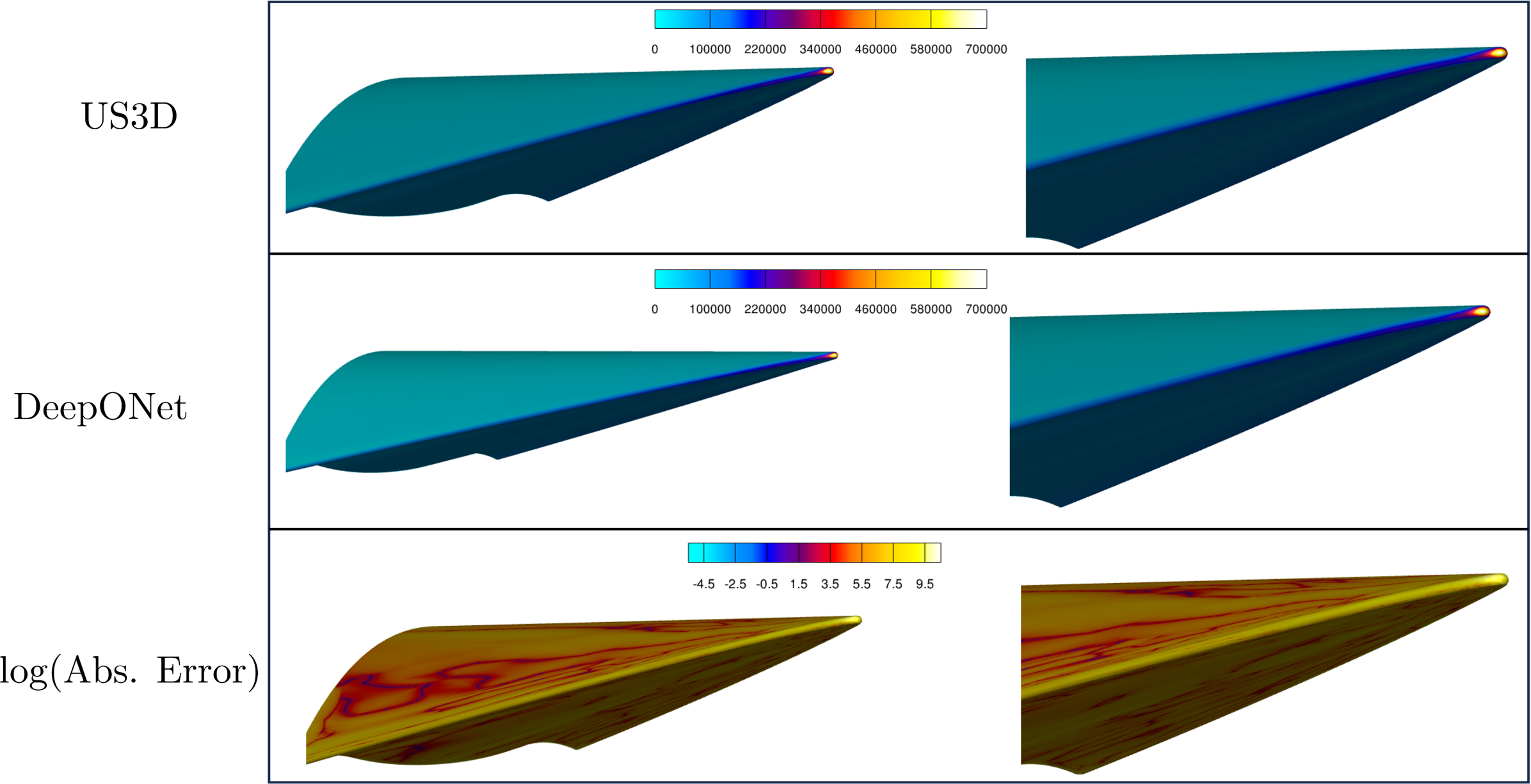
  Figure 5: Heat flux ($Q_w$) distributions on the surface of the AEDC waverider. We compare the fields simulated by the US3D solver against those predicted by the surrogate DeepONet for an unseen 2^∘ angle of attack.

  3.3 Hypersonic Waverider Study for Volume Quantities

  We employ the two-step method outlined in subsubsection 2.1.2 to train a DeepONet for the flow fields across the entire volume. The data generation process mirrors that of the scenario detailed in subsection 3.2. However, in this instance, we used a larger dataset encompassing angles of attack with 1-degree increments ranging from $-{14}^{\circ }$ to $+{14}^{\circ }$, resulting in a total of 29 AoAs. Of these 29 angles, 20 were used for training and 9 were set aside for testing. Subsequently, we proceed to compare the density ($\rho$) field simulated by the US3D solver with the predictions generated by the surrogate 3D DeepONet across the entire domain. Because the input to the volume DeepONet is the set of approximately 50.76 M grid node locations, it necessitates a deeper neural network to converge.

  In Figure 6, the density ($\rho$) distribution at a 3^∘ angle of attack is shown for the entire fluid domain encompassing the AEDC waverider. The first, second and third column in in Figure 6 illustrate the density simulated by the US3D solver, predicted by the two-step DeepONet, and the pointwise error, respectively. However, in the fourth and fifth columns, we present density slices in the XY and YZ planes obtained from the US3D solver and DeepONet, respectively. In the sixth column of Figure 6, we show the pointwise absolute error between the density slices obtained from US3D and DeepONet, respectively. Notably, as depicted in Figure 6, the two-step DeepONet effectively captures the shock location in the flow fields. The global relative error between the numerical and predicted density is 5.1%. Additionally, the inference time for predicting the flow field using the trained DeepONet is 1.032 ms on an A100 NVIDIA GPU, significantly faster than the wall time taken by the US3D solver, which amounts to 32,000 core hours.

  

  

  Figure 6: Density ($\rho$) distributions of the fluid domain around an AEDC waverider for an unseen 3^∘ angle of attack. From left to right the first three columns are: the flow field predicted by the US3D solver; the flow field predicted by the surrogate two-step DeepONet; and the pointwise error (difference) between the US3D solve and DeepONet flow field predictions across the entire volume. The last three columns are slices of the density distribution from left to right: the flow field predicted by the US3D solver; the flow field predicted by the surrogate two-step DeepONet; and the pointwise absolute error (absolute difference) between the US3D solve and DeepONet flow field predictions.

  In Table 1, we show all the hyper-parameters used in generating the results shown in Figure 4, Figure 5 and Figure 6.

  Table 1: Hyperparameters for the experiments in this study, referenced by figure number.

  Figure No.	No. of Hidden Layers	No. of Neurons in each layer	Activation function
  Figure 4	Branch Net = 2, Trunk Net=2	Branch Net = 100, Trunk Net=100	Tanh
  Figure 5	Branch Net = 2, Trunk Net=3	Branch Net = 64, Trunk Net=64	ReLu
  Figure 6	Branch Net = 8, Trunk Net=8	Branch Net = 48, Trunk Net=48	ReLu

  4 Summary and Conclusions

  We have successfully developed surface and volume DeepONet based surrogate models of the AEDC Waverider under hypersonic flow conditions. To address capturing the position of shocks and other areas of high gradients, we use the two-step training method for DeepONets. The two-step method ensures the selection of appropriate basis functions, resulting in improved convergence and accuracy. It offers a reduced training cost advantage compared to the vanilla DeepONet, as it separately trains the branch and trunk networks. We empirically validate the effectiveness of DeepONets in maintaining sufficient accuracy in flow field representation while significantly enhancing computational efficiency compared to using traditional CFD solvers. This enhancement makes DeepONets suitable for various engineering applications, including shape optimization.

  Crucially, DeepONets demonstrate minimal generalization error across the dataset, enabling accurate prediction of the flow field with approximately a 32,000-fold speed-up compared to the CFD baseline. However, mitigating the computational complexity associated with training a DeepONet can be achieved by seamlessly extending the training procedures across multiple GPUs in a data-parallel sense, as outlined in [41]. The framework presented here is versatile and capable of tackling more intricate issues involving multiple inputs, such as varying Mach numbers and diverse parameterizations of geometry, which can be fed into either the branch or trunk networks. Consequently, with minor adjustments, this framework can accommodate optimization in high-speed flow regimes characterized by flow unsteadiness, shocks, non-equilibrium chemistry, and even adaptive geometry. The future work includes integration of CFD surrogate with optimization packages such as Dakota for concept evaluation.

  Acknowledgments

  Copyright 2024 Carnegie Mellon University, Khemraj Shukla, Luis Bravo, Nicholas Plewacki, Anindya Ghoshal, George Karniadakis. This material is based upon work funded and supported by the Department of Defense under Contract No. FA8702-15-D-0002 with Carnegie Mellon University for the operation of the Software Engineering Institute, a federally funded research and development center, and by DEVCOM Army Research Laboratory grants, 185 W911NF-19-1-0225 and W911NF-22-2-0058.

  [DISTRIBUTION STATEMENT A] This material has been approved for public release and unlimited distribution.

  The authors gratefully acknowledge the High-Performance Computing Modernization Program (HPCMP) resources and support provided by the Department of Defense Supercomputing Resource Center (DSRC) as part of the 2022 Frontier Project, Large-Scale Integrated Simulations of Transient Aerothermodynamics in Gas Turbine Engines.

  The views and conclusions contained in this document are those of the authors and should not be interpreted as representing the official policies or positions, either expressed or implied, of the DEVCOM Army Research Laboratory or the U.S. Government.

  This work is licensed under a Creative Commons Attribution-Non Commercial 4.0 International License.

  Requests for permission for non-licensed uses should be directed to the Software Engineering Institute at permission@sei.cmu.edu.

  The U.S. Government is authorized to reproduce and distribute reprints for Government purposes notwithstanding any copyright notation herein. DM23-2250

  References

  • De et al. [2022]
• De, S., Hassanaly, M., Reynolds, M., King, R. N., and Doostan, A., “Bi-fidelity Modeling of Uncertain and Partially Unknown Systems using DeepONets. Preprint at https://arxiv.org/abs/2204.00997,” , 2022. 10.48550/ARXIV.2204.00997.
• Howard et al. [2022]
• Howard, A. A., Perego, M., Karniadakis, G. E., and Stinis, P., “Multifidelity Deep Operator Networks. Preprint at https://arxiv.org/abs/2204.09157,” , 2022. 10.48550/ARXIV.2204.09157.
• Lu et al. [2022a]
• Lu, L., Pestourie, R., Johnson, S. G., and Romano, G., “Multifidelity deep neural operators for efficient learning of partial differential equations with application to fast inverse design of nanoscale heat transport,” Phys. Rev. Research, Vol. 4, 2022a, p. 023210.
• Jin et al. [2022]
• Jin, P., Meng, S., and Lu, L., “MIONet: Learning multiple-input operators via tensor product,” arXiv preprint arXiv:2202.06137, 2022.
• Zhu et al. [2022]
• Zhu, M., Zhang, H., Jiao, A., Karniadakis, G. E., and Lu, L., “Reliable extrapolation of deep neural operators informed by physics or sparse observations,” arXiv preprint arXiv:2212.06347, 2022.
• Hesthaven and Ubbiali [2018]
• Hesthaven, J. S., and Ubbiali, S., “Non-intrusive reduced order modeling of nonlinear problems using neural networks,” Journal of Computational Physics, Vol. 363, 2018, pp. 55–78.
• Hesthaven et al. [2016]
• Hesthaven, J. S., Rozza, G., Stamm, B., et al., Certified reduced basis methods for parametrized partial differential equations, Vol. 590, Springer, 2016.
• Benner et al. [2017]
• Benner, P., Ohlberger, M., Patera, A., Rozza, G., and Urban, K., Model reduction of parametrized systems, Springer, 2017.
• Williams et al. [2015]
• Williams, M. O., Kevrekidis, I. G., and Rowley, C. W., “A data–driven approximation of the koopman operator: Extending dynamic mode decomposition,” Journal of Nonlinear Science, Vol. 25, No. 6, 2015, pp. 1307–1346.
• Chiavazzo et al. [2014]
• Chiavazzo, E., Gear, C. W., Dsilva, C. J., Rabin, N., and Kevrekidis, I. G., “Reduced models in chemical kinetics via nonlinear data-mining,” Processes, Vol. 2, No. 1, 2014, pp. 112–140.
• Lieberman et al. [2010]
• Lieberman, C., Willcox, K., and Ghattas, O., “Parameter and state model reduction for large-scale statistical inverse problems,” SIAM Journal on Scientific Computing, Vol. 32, No. 5, 2010, pp. 2523–2542.
• Bui-Thanh et al. [2008]
• Bui-Thanh, T., Willcox, K., and Ghattas, O., “Model reduction for large-scale systems with high-dimensional parametric input space,” SIAM Journal on Scientific Computing, Vol. 30, No. 6, 2008, pp. 3270–3288.
• Benner et al. [2015]
• Benner, P., Gugercin, S., and Willcox, K., “A survey of projection-based model reduction methods for parametric dynamical systems,” SIAM review, Vol. 57, No. 4, 2015, pp. 483–531.
• Amsallem et al. [2015]
• Amsallem, D., Zahr, M., Choi, Y., and Farhat, C., “Design optimization using hyper-reduced-order models,” Structural and Multidisciplinary Optimization, Vol. 51, No. 4, 2015, pp. 919–940.
• Carlberg and Farhat [2008]
• Carlberg, K., and Farhat, C., “A compact proper orthogonal decomposition basis for optimization-oriented reduced-order models,” 12th AIAA/ISSMO multidisciplinary analysis and optimization conference, 2008, p. 5964.
• Choi et al. [2020]
• Choi, Y., Boncoraglio, G., Anderson, S., Amsallem, D., and Farhat, C., “Gradient-based constrained optimization using a database of linear reduced-order models,” Journal of Computational Physics, Vol. 423, 2020, p. 109787.
• Kammeyer and Gillum [1994]
• Kammeyer, M. E., and Gillum, M. J., “Design Validation Tests on a Realistic Hypersonic Waverider at Mach 10, 14, and 16.5 in the Naval Surface Warfare Center Hypervelocity Wind Tunnel No. 9,” 1994, pp. 93–198.
• Zhang et al. [2021]
• Zhang, X., Xie, F., Ji, T., Zhu, Z., and Zheng, Y., “Multi-fidelity deep neural network surrogate model for aerodynamic shape optimization,” Computer Methods in Applied Mechanics and Engineering, Vol. 373, 2021, p. 113485.
• Zhiwei et al. [2020]
• Zhiwei, S., Chen, W., Zheng, Y., Junqiang, B., Zheng, L., Qiang, X., and Qiujun, F., “Non-intrusive reduced-order model for predicting transonic flow with varying geometries,” Chinese Journal of Aeronautics, Vol. 33, No. 2, 2020, pp. 508–519.
• Renganathan et al. [2021]
• Renganathan, S. A., Maulik, R., and Ahuja, J., “Enhanced data efficiency using deep neural networks and Gaussian processes for aerodynamic design optimization,” Aerospace Science and Technology, Vol. 111, 2021, p. 106522.
• Xing et al. [2022]
• Xing, H., Xiao, Z., Zhan, D., Luo, S., Dai, P., and Li, K., “SelfMatch: Robust semisupervised time-series classification with self-distillation,” International Journal of Intelligent Systems, Vol. 37, No. 11, 2022, pp. 8583–8610.
• Xiao et al. [2021]
• Xiao, Z., Xu, X., Xing, H., Luo, S., Dai, P., and Zhan, D., “RTFN: a robust temporal feature network for time series classification,” Information sciences, Vol. 571, 2021, pp. 65–86.
• Mishra et al. [2022a]
• Mishra, R. K., Choudhary, A., Mohanty, A., and Fatima, S., “An intelligent bearing fault diagnosis based on hybrid signal processing and Henry gas solubility optimization,” Proceedings of the Institution of Mechanical Engineers, Part C: Journal of Mechanical Engineering Science, Vol. 236, No. 19, 2022a, pp. 10378–10391.
• Mishra et al. [2022b]
• Mishra, R. K., Choudhary, A., Fatima, S., Mohanty, A. R., and Panigrahi, B. K., “A self-adaptive multiple-fault diagnosis system for rolling element bearings,” Measurement Science and Technology, Vol. 33, No. 12, 2022b, p. 125018.
• Mishra et al. [2022c]
• Mishra, R., Choudhary, A., Fatima, S., Mohanty, A., and Panigrahi, B., “A Fault Diagnosis Approach Based on 2D-Vibration Imaging for Bearing Faults,” Journal of Vibration Engineering & Technologies, 2022c, pp. 1–14.
• Du et al. [2021]
• Du, X., He, P., and Martins, J. R., “Rapid airfoil design optimization via neural networks-based parameterization and surrogate modeling,” Aerospace Science and Technology, Vol. 113, 2021, p. 106701.
• Hao et al. [2023]
• Hao, Z., Wang, Z., Su, H., Ying, C., Dong, Y., Liu, S., Cheng, Z., Song, J., and Zhu, J., “GNOT: A General Neural Operator Transformer for Operator Learning,” Proceedings of the 40th International Conference on Machine Learning, Proceedings of Machine Learning Research, Vol. 202, PMLR, 2023, pp. 12556–12569.
• Liao et al. [2021]
• Liao, P., Song, W., Du, P., and Zhao, H., “Multi-fidelity convolutional neural network surrogate model for aerodynamic optimization based on transfer learning,” Physics of Fluids, Vol. 33, No. 12, 2021, p. 127121.
• Tao and Sun [2019]
• Tao, J., and Sun, G., “Application of deep learning based multi-fidelity surrogate model to robust aerodynamic design optimization,” Aerospace Science and Technology, Vol. 92, 2019, pp. 722–737.
• Zhao et al. [2023]
• Zhao, T., Qian, W., Lin, J., Chen, H., Ao, H., Chen, G., and He, L., “Learning Mappings from Iced Airfoils to Aerodynamic Coefficients Using a Deep Operator Network,” Journal of Aerospace Engineering, Vol. 36, No. 5, 2023, p. 04023035.
• Lu et al. [2022b]
• Lu, L., Meng, X., Cai, S., Mao, Z., Goswami, S., Zhang, Z., and Karniadakis, G. E., “A comprehensive and fair comparison of two neural operators (with practical extensions) based on fair data,” Computer Methods in Applied Mechanics and Engineering, Vol. 393, 2022b, p. 114778.
• Li et al. [2022]
• Li, Z., Huang, D. Z., Liu, B., and Anandkumar, A., “Fourier neural operator with learned deformations for pdes on general geometries,” arXiv preprint arXiv:2207.05209, 2022.
• Serrano et al. [2023]
• Serrano, L., Vittaut, J.-N., et al., “OPERATOR LEARNING ON FREE-FORM GEOMETRIES,” ICLR 2023 Workshop on Physics for Machine Learning, 2023.
• Vasile et al. [2022]
• Vasile, J. D., Fresconi, F., DeSpirito, J., Duca, M., Recchia, T., Grantham, B., Bowersox, R. D. W., and White, E. B., “High-Speed Army Reference Vehicle,” US Army Combat Capabilities Development Command, Army Research Laboratory, 2022. URL https://apps.dtic.mil/sti/pdfs/AD1176136.pdf.
• Lu et al. [2019]
• Lu, L., Jin, P., and Karniadakis, G. E., “Deeponet: Learning nonlinear operators for identifying differential equations based on the universal approximation theorem of operators,” arXiv preprint arXiv:1910.03193, 2019.
• Lee and Shin [2023]
• Lee, S., and Shin, Y., “On the training and generalization of deep operator networks,” arXiv preprint arXiv:2309.01020, 2023.
• Chen and Chen [1995]
• Chen, T., and Chen, H., “Universal approximation to nonlinear operators by neural networks with arbitrary activation functions and its application to dynamical systems,” IEEE Transactions on Neural Networks, Vol. 6, No. 4, 1995, pp. 911–917.
• Lu et al. [2021]
• Lu, L., Jin, P., Pang, G., Zhang, Z., and Karniadakis, G. E., “Learning nonlinear operators via DeepONet based on the universal approximation theorem of operators,” Nature Machine Intelligence, Vol. 3, No. 3, 2021, pp. 218–229.
• Li et al. [2020]
• Li, Z., Kovachki, N., Azizzadenesheli, K., Liu, B., Bhattacharya, K., Stuart, A., and Anandkumar, A., “Neural Operator: Graph Kernel Network for Partial Differential Equations,” , 2020.
• Candler et al. [2015]
• Candler, G., Johnson, H., Nompelis, I., Gidzak, V., Subbareddy, P., and Barnhardt, M., “Development of the US3D Code for Advanced Compressible and Reacting Flow Simulations,” 53rd AIAA Aerospace Sciences Meeting, 2015. 10.2514/6.2015-1893, URL https://arc.aiaa.org/doi/abs/10.2514/6.2015-1893.
• Goyal et al. [2017]
Goyal, P., Dollár, P., Girshick, R., Noordhuis, P., Wesolowski, L., Kyrola, A., Tulloch, A., Jia, Y., and He, K., “Accurate, large minibatch sgd: Training imagenet in 1 hour,” arXiv preprint arXiv:1706.02677, 2017.