 |
| The geometry of SAR platforms for the tomo-SAR process |
A Robust Super-resolution Gridless Imaging Framework for UAV-borne SAR Tomography
Synthetic aperture radar (SAR) tomography (TomoSAR) retrieves three-dimensional (3-D) information from multiple SAR images, effectively addresses the layover problem, and has become pivotal in urban mapping.
Unmanned aerial vehicle (UAV) has gained popularity as a TomoSAR platform, offering distinct advantages such as the ability to achieve 3-D imaging in a single flight, cost-effectiveness, rapid deployment, and flexible trajectory planning. The evolution of compressed sensing (CS) has led to the widespread adoption of sparse reconstruction techniques in TomoSAR signal processing, with a focus onℓ1 norm regularization and other grid-based CS methods. However, the discretization of illuminated scene along elevation introduces modeling errors, resulting in reduced reconstruction accuracy, known as the "off-grid" effect. Recent advancements have introduced gridless CS algorithms to mitigate this issue.
This paper presents an innovative gridless 3-D imaging framework tailored for UAV-borne TomoSAR. Capitalizing on the pulse repetition frequency (PRF) redundancy inherent in slow UAV platforms, a multiple measurement vectors (MMV) model is constructed to enhance noise immunity without compromising azimuth-range resolution.
Given the sparsely placed array elements due to mounting platform constraints, an atomic norm soft thresholding algorithm is proposed for partially observed MMV, offering gridless reconstruction capability and super-resolution. An efficient alternative optimization algorithm is also employed to enhance computational efficiency. Validation of the proposed framework is achieved through computer simulations and flight experiments, affirming its efficacy in UAV-borne TomoSAR applications.
| Subjects: | Signal Processing (eess.SP) | |
| Cite as: | arXiv:2402.01194 [eess.SP] | |
| (or arXiv:2402.01194v1 [eess.SP] for this version) |
Summary
The key points are:
- The paper proposes a robust gridless 3D imaging framework called EMPAST for UAV-borne SAR tomography. The framework has superior super-resolution capability and noise immunity.
- It constructs multiple measurement vectors (MMV) from oversampled SAR data by extracting along the slow time, utilizing the narrow Doppler bandwidth of UAV platforms. This enhances noise resilience without compromising resolution.
- It accounts for sparse arrangement of array elements on UAVs. An atomic norm soft thresholding algorithm is proposed for sparse reconstruction from partial MMV observations. This provides gridless estimation and mitigates off-grid effects.
- An efficient ADMM optimization method is presented to solve the large-scale semidefinite programming problem for atomic norm minimization.
- The framework is validated on simulated and real measured data from flight experiments using a UAV-borne tomography SAR system called MV3DSAR. It demonstrates superior performance in accuracy, noise robustness, super-resolution and efficiency compared to other methods.
- The technique allows high-quality 3D point cloud reconstruction of buildings from UAV-borne TomoSAR data, with applications in urban mapping.
EMPAST framework
Here is a more detailed summary of the EMPAST framework:
- EMMV Construction: It extracts multiple measurement vectors (MMV) from oversampled SAR data by retaining certain slow-time samples based on the PRF. This is done by extracting along slow time direction while ensuring full azimuth-range resolution.
- Atomic Norm Soft Thresholding Algorithm: It defines a new atomic norm for the partial MMV case. The atomic norm denoising problem is posed as optimization and solved via semidefinite programming. A new regularization parameter selection method is proposed.
- Efficient Optimization Using ADMM: To solve the large-scale SDP efficiently, an Alternating Direction Method of Multipliers (ADMM) approach is presented. It involves iterative updates of variables based on augmented Lagrangian.
- Steps of EMPAST:
- Construct EMMV from oversampled data
- Perform tomography on EMMV using proposed algorithm
- Initialize ADMM variables and parameters
- Iterate ADMM steps of variable updates and multipliers
- Extract target locations from optimizer matrix using Vandermonde decomposition
- Fuse TomoSAR point cloud with LiDAR data for visualization
- Benefits:
- Improves noise resilience through MMV
- Provides super-resolution via gridless atomic norm
- Computationally efficient compared to standard SDP solvers
- Mitigates off-grid effects that degrade standard CS methods
- Allows high quality 3D reconstruction from UAV data
In summary, the key innovation of EMPAST is the extraction of MMV from UAV data and a tailored gridless reconstruction algorithm that provides state-of-the-art performance.
Authors
Author Background:
The authors have strong expertise in SAR signal processing and remote
sensing, with access to unique UAV-SAR data artifacts that enabled
development and validation of the EMPAST framework.
- The authors are researchers affiliated with various institutions in China, including
- Aerospace Information Research Institute,
- Chinese Academy of Sciences,
- University of Chinese Academy of Sciences,
- Xi'an Jiaotong University, and
- Suzhou Institute of Nano-Tech and Nano-Bionics.
- Many of the authors are affiliated with radar, remote sensing and signal processing research groups/labs, indicating background and expertise in these areas.
Related Publications:
- First author Silin Gao has a publication titled "Robust Superresolution DOA Estimation Based on Sparse Bayesian Learning" in IEEE Signal Processing Letters in 2022.
- Co-author Zhe Zhang has publications on topics like SAR imaging, radar signal processing, and compressive sensing.
- Senior author Xiaolan Qiu has extensive publications on radar imaging and remote sensing.
Institutions:
- Key institutions involved are Aerospace Information Research Institute, Chinese Academy of Sciences, Xi'an Jiaotong University, and Suzhou Institute of Nano-Tech and Nano-Bionics.
- The research is associated with various state key labs and research institutes within the Chinese Academy of Sciences.
Artifacts:
- The framework is validated on data from the MV3DSAR system, an experimental UAV-borne array SAR platform developed by the Aerospace Information Research Institute.
- Simulated data is also used to validate the approach and compare performance.
- The technique is applied on measured data from flight experiments conducted using the MV3DSAR system in Tianjin, China. This provided real 3D SAR data of buildings to reconstruct point clouds.
MV3DSAR system
MV3DSAR stands for Microwave-Vision 3D Synthetic Aperture Radar. It is an experimental small UAV-borne array SAR system developed by the Aerospace Information Research Institute, Chinese Academy of Sciences.
Key details about MV3DSAR:
- Platform: Small fixed-wing unmanned aerial vehicle (UAV)
- Configuration: 2 transmit antennas and 2 receive antennas forming 4 equivalent antenna phase centers in linear array configuration.
- Frequency band: Ku band (specifically 15.2 GHz)
- Modes: Stripmap mode, spotlight mode
- Resolution: High resolution in azimuth, range and elevation
- Processing: Digital beamforming and tomography processing
- Applications: High-resolution 3D imaging, urban mapping
MV3DSAR is designed specifically to provide 3D tomographic capabilities on a small UAV platform. The multiple antenna phase centers allow aperture synthesis in elevation and multi-baseline tomography.
The system parameters are provided in the paper:
- 400 m altitude,
- 15.2 GHz center frequency,
- 1 kHz PRF,
- 4 equivalent apertures,
- 0.54 m elevation aperture.
The EMPAST framework proposed in the paper is validated on measured data from flight experiments conducted using MV3DSAR over buildings in Tianjin, China. This provided real measured data to verify the 3D tomography and imaging capabilities.
In summary, MV3DSAR is a custom-built UAV-SAR system with array configuration to enable high-resolution 3D SAR imaging and tomography, suitable for applications like urban mapping.
A tutorial on tomographic synthetic aperture radar methods
1 Introduction
In the late 1940s, after the second world war, the United States army was looking for an all-weather, 24-h remote surveillance device. The ability of the radar to penetrate cloud and fog and its independence from daylight made it the logical choice for the army. The only issue was that in order to achieve a high enough resolution the antenna would need to be the size of a football field, far too large for any aircraft to carry. Synthetic aperture radar (SAR) was the solution to this problem. It was invented by Carl A. Wiley, a mathematician at Goodyear Aircraft Company, in 1951. This technology was released to the civilian communities in the 1970s. This type of radar increases the resolution by using the movement of the platform to create a synthetic aperture.
SAR stores the data of the scanned area in the form of a 2-dimensional signal (similar to an image); however, the actual landscape is 3-dimensional. Therefore, SAR in fact maps the information of the 3-dimensional area into two dimensions. During this mapping process, not only we lose the data for the third dimension, but also since the model is summed in one direction, it becomes less accurate. The process of tomography aims to untangle this mapped version of the landscape and estimate the original 3-dimensional model by calculating the reflectivity and elevation of the scatterers using multiple SAR acquisitions. Any object or surface that comes into contact with the beam scatters the signal in all direction which is why we use the term “scatterer” to describe them. The goal of this study is to create a tutorial for the SAR tomography (tomo-SAR) process using real SAR data. To this end, in the second section, we discuss what SAR is and introduce some of the most famous platforms on which SAR equipment are mounted. The third section covers what tomo-SAR is and the mathematical modeling and equations supporting this method. The fourth section includes all the preprocessing steps required for SAR data processing and the tomography process. All the necessary information about the required dataset is included in the fifth section. The sixth section includes several different spectral estimation strategies that are currently being used in the tomo-SAR process. In the seventh and final section we have the conclusions and the possible future topics for research in this field.
2 Synthetic aperture radar
SAR is a type of imaging radar that has many applications, from agriculture to military. This type of radar is usually mounted on a moving platform such as an aircraft or spacecraft and is, in fact, an advanced form of side-looking-airborne radar (SLAR). The size of the antenna or the antenna aperture is in direct relation with the image resolution; which means the larger the antenna aperture is, the higher the image resolution will be. In Ponce et al. [1], published a transaction paper on holographic SAR tomography where they discuss the synthesized aperture of SAR in details. For this type of radar, the movement of the platform at high speed acts as another form of antenna aperture. The combination of the aperture caused by the movement of the platform and the physical antenna aperture create a synthetic aperture which is capable of achieving a higher resolution than would be possible for the physical antenna of the radar by itself [2]. SAR has three modes of acquisition, stripmap, spotlight and scanSAR modes. In the strip map mode the transmitter is fixed; therefore, the beam scans a swath parallel to the azimuth axis. In the scanSAR mode, the transmitter moves orthognal to the azimuth direction and the swath will creating zigzags on the ground. In this mode the scanned area increases but since the scan time is decreases, the final resolution would be also decrease. In the spotlight mode the transmitter moves in the direction of azimuth axis to keep the beam focused on one location as long as possible. In this mode the scanned area is reduced considerably but the since the scan time is increased, the resolution would be higher. The three SAR acquisition modes are shown in Fig. 1.
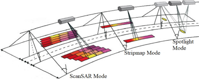
SAR acquisition modes (Spotlight, Stripmap and ScanSAR) [3]
The data from each transmit/receive cycle is a complex signal and is stored as amplitude and phase. After a given number of cycles, the stored data are combined to create a single high-resolution image [4]. By using SAR it is possible to create a signal which would have been obtained by an antenna of length V.T; where T is the time period, and V is the speed of the platform. When an object enters the radar beam, the echoes from each transmitted pulse are recorded while the platform continues to move forward, and keeps recording all the echoes until the object leaves the beam. The velocity of the platform and the time the object is in the sight of the radar, determine the length of the simulated and synthesized aperture. In Soumekh [5] published a book on SAR signal processing which includes the basic and traditional SAR signal analysis techniques. In Table 1 we have included some examples of several airborne platforms that are equipped with SAR. In this table the band, polarization, look angle and several other specifications of eleven SAR platforms are demonstrated.
3 SAR tomography
The traditional SAR acquisitions are not only missing the third dimension, but also suffer from the “layover phenomenon”. If the range and azimuth resolution of a SAR acquisition is \(m \times n\), every scatterer in this area contributes to the final complex value of the pixel [6]. As it can be seen form Fig. 2, Slant-range is the distance from the scatterers to the radar; therefore, every object that has the same distance from the radar will contribute to the complex value of the same pixel, this phenomenon is known as layover and it causes great inaccuracies in the pixel values [7].
Tomo-SAR is an advanced signal processing method that uses multiple 2-dimensional SAR acquisitions of the same area to calculate the elevation of each of the scatterers contributing to the values of each pixel. Each of the different scatterers with different elevations, have different reflectivity coefficients. Tomo-SAR uses spectral estimation methods to calculate the elevation and reflectivity pairs of each of the scatterers within the pixels. For each pixel, the SAR measurements are in fact the sampled Fourier transforms of the reflectivity function [9]. In Pardini and Papathanassiou [10] improved the performance of capon beamformer spectral estimator method by using proir information about the topography of the landscape.
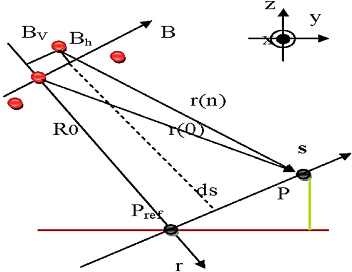
Figure 3 shows the different positions of the radar in relation to the scatterer at position \(\textit{s}\). In this figure the distance between the point \(\textit{s}\) and \(P_{ref}\) is the elevation of this scatterer (which the tomo-SAR method aims to estimate), \(\textit{x}\) represents the flight direction of the platform (azimuth) and \(\textit{r}\) represents the slant-range axis. During the tomo-SAR process, one of the acquisitions is considered to be the master and the rest are considered to be slaves. The horizontal and vertical distances of the position of each slave acquisition from the master position are known as the baseline and are shown by \(B_{h}\) and \(B_{v}\). Only the baseline in the direction of the elevation or \(B_{h}\) is used in the tomo-SAR process and the maximum of of this baseline is shown as \(\textit{B}\) [11]. All these variables can be seen in Fig.3.
$$\begin{aligned} g_n=\int _{\varDelta s} \gamma (s) e^{(-i2\pi f_n s)} ds \end{aligned}$$
(1)
In (1), \(\gamma (s)\) is the continuous reflectivity function along the elevation axis, \(f_n\) is the elevation frequency and \(g_n\) is the Fourier transform of the reflectivity function along elevation at position \(\textit{s}\) [7]. Elevation frequency can be calculated using (2) [12].
$$\begin{aligned} f_n= \frac{-2b_n}{r\lambda } \end{aligned}$$
(2)
In (2) \(b_n\) is the baseline in the direction of elevation, r is the value of range and \(\lambda\) is the wavelength of the radar. If the elevation points are considered to be \(\textit{L}\) discrete, (1) changes to (3).
$$\begin{aligned} g_n=\delta _s\sum _{l=1} ^L \gamma (s) e^{(-2\pi f_n s_l)} ds \end{aligned}$$
(3)
In (3), \(\gamma (s)\) is the discrete reflectivity function along the elevation axis, \(s_{l}\) is the elevation of the \(l_{th}\) scatterer within this pixel (at discrete locations), and \(\delta _s\) is the discretization interval. Therefore, finding the elevation and the reflectivity of each scatterer within the pixel becomes an spectral estimation problem . In Sect. 6, we will describe several algorithms for solving this spectral estimation problem.
4 Tomo-SAR data preprocessing
As we mentioned previously, SAR acquisition is in the form of multiple 2-dimensional complex signals. These complex signals along with other related data, are contained within specific data packet. To access the data within these packets we must use certain softwares and toolboxes. For the case of Sentinel-1a data packets, we must use the sentinel application platform (SNAP), which is a software that contains all sentinel toolboxes. We have used this software for accessing and processing of our raw data packets.
Every data packet is divided into four parts, metadata, vector data, tie-point grids, and bands. The band section of the data packets contains the scan signal of the landscape which is the main part of the data; the other sections hold other essential information. For the data packets that we have used in this study, the band section of each data packet contains three acquisition of the landscape. Each of the acquisitions in the band section has two polarization where each polarization contains three sub-swaths. Therefore there are a total of eighteen files within the band section of each of the acquired data packets. This number can be different for different modes of acquisition. The first file or \(\textit{I}\) represents the real part, while the second file or \(\textit{Q}\) represents the imaginary part of the complex image. The third file is the intensity of the other two images and is not necessary for the tomo-SAR process. In order to use these files for estimation of elevation, they must first go through several preprocessing steps.
4.1 Radiometric calibration
The different software and processor usually apply their own scaling based on the equipment or application. The radiometric calibration step of preprocessing, undoes the previously applies calibration and applies new calibration on all acquisitions therefore unifying them for the tomo-SAR process. This step can be done using the SNAP toolbox where it uses the four calibration look up tables (LUT) inside each data packet to perform the radiometric calibration on all acquisitions. This step is applied to enable fair comparison between different sensors, processors, modes etc. and therefore it is a necessary part of the tomo-SAR preprocessing [13, 14]. The mathematical equation of radiometric calibration is given in (4).
$$\begin{aligned} K_i = \frac{|DN_i|^2}{A_i} \end{aligned}$$
(4)
In (4), \(A_i\) represents the backscattering coefficient of the pixel area and can be expressed in the slant-range plane (beta nought), on the ground (sigma nought), or in the plane perpendicular to the slant-range direction (gamma nought). Digital number (DN) represents the pixel intensity of the \(i^{th}\) pixel of the image, and \(k_i\) is the absolute calibration constant [15]. Since our objective is to use multiple images, all of our images must be calibrated. We have performed this step using the Sentinel-1 toolbox of SNAP software and have applied calibration on all of the images of the dataset.
4.2 Coregistration
In tomo-SAR, acquisitions are taken from different angles and are moved compared to each other, which means a specific pixel in different acquisitions (for instance, pixel \(50 \times 50\) of each image) no longer indicates a certain point on the ground. Image coregistration aligns one or more slave acquisition with the master in such a way that each pixel from the coregistered slave image represents the same point on the Earth’s surface as its corresponding pixel in the master image. This process is an essential part of the tomo-SAR and Interferometric SAR (In-SAR) process. To obtain a high-quality In-SAR image, the individual complex images need to be coregistered to sub-pixel accuracy [16]. In Plyer et al. [17] developed a novel algorithm that was able to reduce the coregistration error to 0.1 pixel between stripmap and spotlight acquisitions and 0.7 pixel between two spotlight acquisitions. In this project we have used terrain observation with progressive scans SAR (TOPSAR) which will be explained in details in the fifth section. The coregistration of TOPSAR sigals is accomplished in three major processing steps. A simple diagram of this process can be seen in Fig. 4.
- 1.TOPSAR-Split
- 2.Apply-Orbit-File
- 3.Back-Geocoding
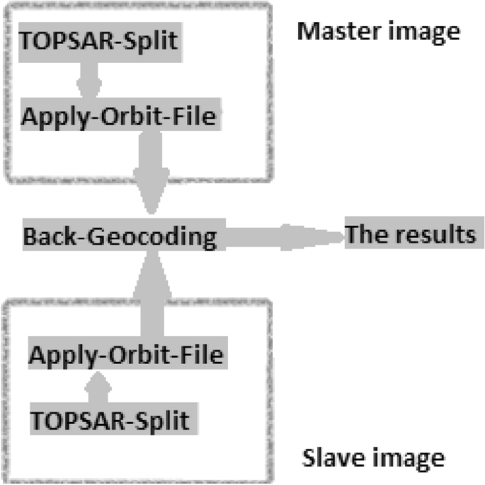
The schematic of TOPSAR coregistration process
In the TOPSAR-Split step, each sub-swath is split into a separate signal. In the second step of coregistration the precise orbit file is applied to the data. The orbit state vectors provided in the metadata of the SAR data packets are generally not accurate enough; therefore, the precise orbit files must be used to refine them. The precise orbit files are available in the database, days (in some cases weeks) after the generation of the product. Each data has an orbit file which must be acquired separately. The orbit file provides accurate satellite position and velocity information. Based on this information, the orbit state vectors in the abstract metadata of the product are updated. However, since the precise orbit file of a Sentinel-1a data packet is only available for twelve months or less, many of our acquired data packets were unusable. There are other types of orbit files available for these images; however, since tomography is a very precise process using these types of orbit files will introduce a significant amount of noise to the results.
Back-Geocoding is the last major step in TOPSAR coregistration. In this step, two single look complex (SLC) split products (master and slave) of the same sub-swath will be coregistered using the orbits of the two products and an external digital elevation model (DEM). In resampling slave image into the master frame, first deramping and demodulation are performed to the slave image, and then the truncated-sinc interpolation is performed. Finally, the reramp and remodulation are applied to the interpolated slave image.
To perform the coregistration process, we used the SNAP toolbox; however, in this program, it is only possible to coregister one slave with one master data packet. In order to coregister all acquisitions with a single master image, first, we have to find the optimum master acquisition of the dataset. The master image is selected such that the dispersion of the perpendicular baseline is as low as possible. During the coregistration process the master data will not change at all, and all the changes will be applied to the slave images. If all the slave images are coregistered with respect to a single master image, it means all images are coregistered with each other. After this process all pixels of the same location (row and column) in every image in a data stack, will point to the exact same location on the ground.
4.3 Debursting
As it was mentioned, each Sentinel-1a TOPSAR interferometric wide swath (IW) SLC data packet consists of two polarizations; where each polarization consists of three sub-swaths. Each of the mentioned sub-swaths consists of several bursts, where each burst was processed as a separate SLC image. To create level-2 data, these bursts will merge through the multi-looking process and form a single image; however, for the tomography process, only one acquisition per image can be used. Therefore before the tomography process, the different burts of each sub-swath must be separated. We have used the deburst operator of the SNAP toolbox to deburst all sub-swaths in our dataset. Debursting and splitting are two completely different steps and must not be mistaken with each other; Splitting is an operator that splits a certain sub-swath from the whole data; however, as it was explained, debursting is an step in which different bursts are separated within each sub-swath. After the debursting step, a specific area of each image will be chosen. We have collected pixels 18,500 up to 19,000 of the \(\textit{x}\) axis and 5500 up to 6000 of the \(\textit{y}\) axis of all images in our data stack. At this point, our dataset is ready to be imported to the Matlab program for further analysis.
5 Tomo-SAR dataset
SAR data is not easily available, which makes finding a tomo-SAR dataset extremely difficult. Therefore in many cases it may be easier to create a tomo-SAR dataset from raw SAR data. The first important issue when creating tomo-SAR dataset is to use SLC split images. As it was briefly mentioned in the previous section, after creating the level-1 SLC splits from the level-0 raw signals, it is possible to create the level-2 signals using the multi-looking and ground range detection (GRD) process. These images can no longer be used in radar processing because the phase information is lost during the multi-looking process. The level-2 signals are in the image domain and no longer represent the complex Fourier transforms of the reflectivity function; therefore we can only use SLC data for the tomography process. In Fig.5 we can see a small portion of an SLC image from the dataset; all the three images represent one SLC signal (real, imaginary and intensity). Figure6 shows the level-2 image of the same area as Fig. 5, after the multi-looking and GRD process.
A small portion of a Single Look Complex image a this is the real part of the image b imaginary part of the image c intensity of the SLC image
Level-2 image of the SLC signal of Fig. 5
To create a dataset consisted of SLC data, we have contacted many facilities and individuals, and all of them refused to answer or simply refused except for one, Alaska satellite facility (ASF), who kindly gave us permission to use their database. ASF has an open-source database consisted of data packets from several different satellites. We have gathered several TOPSAR IW data packets from the Sentinel-1a satellite. The TOPSAR technique is a form of scanSAR imaging mode, where data is acquired in bursts by cyclically switching the antenna beam between multiple adjacent sub-swaths. TOPSAR acquisitions can provide large swath widths and enhanced radiometric performance by reducing the scalloping effect. In TOPSAR acquisition method, for each burst, the beam of the radar is steered in the azimuth direction as well as ground range; this reduces the scalloping phenomenon considerably and increases the uniformity of the image quality throughout the swath [18]. TOPSAR mode is intended to replace the conventional scanSAR mode, achieving the same coverage and resolution as scanSAR, but with a nearly uniform signal to noise ratio (SNR) and distributed target ambiguity ratio (DTAR). One of the differences between TOPSAR imaging mode and the conventional scanSAR is the direction of the zigzagging. As it was mentioned before, in scanSAR, the sensor moves in the form of zigzags perpendicular to the direction of the flight to cover more land; TOPSAR sensor does the same movement, but the direction of the zigzags is parallel to the fight path. The disadvantage is that this parallel zigzagging will cause less resolution in the azimuth direction.
We have created a dataset with 4 data packets that satisfy these conditions; however, initially, we acquired more than ten packet of the region, but not all of the acquisitions met the requirements (such as orbit files). Each of the downloaded TOPSAR IW packets covers an area of approximately \(100 \times 60\) km, which by a \(5 \times 25\) resolution gives eighteen 2-dimensional signals with the size of \(20{,}000 \times 12{,}000\) pixels; this is why each of the downloaded data packets has a size of over four gigabytes. More than twenty gigabytes of data were used to create our dataset with these four images. Our dataset contains data packets form the area of Bakersfield in California, United States; the specification of these data packets such as track number or spatial and temporal baselines can be seen in Table 2. The name of a data packet gives a brief description of that dataset, to find more information about the naming conventions visit the European space agency (ESA) website [19]. As it was mentioned, the acquisition that creates the lowest overall spatial baseline with others is chosen as the master image. All acquisitions must have the same track number to be valid for tomo-SAR process, which in Table 2 that number is 144; this means not only the acquisitions are from the same spot on the ground but they are also parallel.
6 Spectral estimation strategies for Tomo-SAR
The main part of tomo-SAR is to solve the spectral estimation problem. The equation of the tomo-SAR model is underdetermined, therefore, it is necessary to use parameter estimation methods to find the reflectivity and elevation of all scatterers of each pixel. In this section we have included five of the most important and well-known spectral estimators used for the tomo-SAR process. We have implemented these methods using Matlab and will demonstrate their results on our dataset in this section.
Many researchers are currently working on new ideas to develop or adapt existing spectral estimation methods for tomo-SAR. In Fabrizio et al. [20] used an adaptive approach to the capon spectral estimation method to increase the resolution of tomo-SAR signals in cases with a limited number of baselines. In Schmitt et al. developed a maximum likelihood based approach which would provide higher resolution even for limited number of baselines [21]. In Becerra et al. [22] used a novel non-parametric spectral analysis approach to increase the resolution and reduce the artifacts.
A \(500 \times 500\) pixels portion of our dataset was chosen, which with the resolution of \(5 \times 25\) m points to an area of 31.25 km\(^2\) on the ground. We have cropped a small part of the whole signals with the size of \(20 \times 20\) to use for demonstration in this section. Due to the limitation of our dataset we have been able to find the maximum of two scatterers per pixel. The layover phonamenon only occurs for a limited number of pixels and having three scatterer in one pixel rarely happens, which is why even with limited amount of data, we can still use the spectral estimation methods to find the elevation. We have used each algorithm for both noisy and denoised data.
6.1 Conventional beamforming
Beamforming technique was the first method that was used for solving the layover problem. If (3) is written for all pixels, the overall system can be written in the form of a matrix equation as in (5).
$$\begin{aligned} \begin{bmatrix} g_0 \\ \vdots \\ g_{n_L} \end{bmatrix} = \begin{bmatrix} e^{-i2\pi f_0 s_1} &{} \cdots &{} e^{-i2\pi f_0 s_{n_L}} \\ \vdots &{}\ddots &{} \vdots \\ e^{-i2\pi f_{n_s} s_1} &{} \cdots &{} e^{-i2\pi f_{n_s} s_{n_L}} \end{bmatrix} . \begin{bmatrix} \gamma _1 \\ \vdots \\ \gamma _{n_L} \end{bmatrix} + \begin{bmatrix} v_0 \\ \vdots \\ v_{n_L} \end{bmatrix} \end{aligned}$$
(5)
The main equation of tomo-SAR can be described as (5) and in compact form it can be rewritten as (6).
$$\begin{aligned} g= R(S)\cdot \gamma \ ,S= \begin{bmatrix} s_1& \cdots&s_{n_p} \end{bmatrix} \end{aligned}$$
(6)
In (6), S is the vector containing the discrete elevation points, \(\gamma\), is the reflectivity vector and R is the measurement matrix, which in case has the form of Fourier transform. The beamforming method simply applies an inverse Fourier transform to the irregularly sampled signal as it can be seen in (7).
$$\begin{aligned} {\hat{\gamma }}= R^{\dagger }(S)\cdot g \end{aligned}$$
(7)
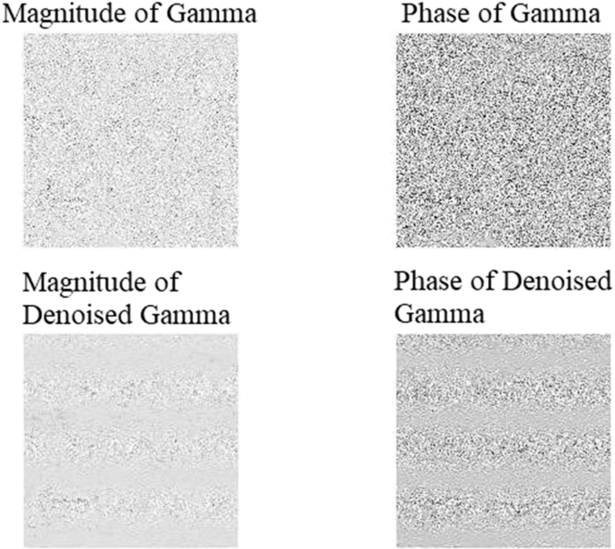
In (7), \(R^{\dagger }\) is the inverse of R and \({\hat{\gamma }}\) is the estimated value for gamma vector. This method is computationally very conventional; however, because it is suffering form a severe side-lobe problem, the error is high. Figures 7 and 8 demonstrate the results of the algorithm for the reflectivity and elevation, respectively; however, as it can be seen in these figures, for this dataset, the results were not acceptable. The equation of most pixels could not be solved, and many singularities were created, which resulted in a discontinuity in elevation. Here we have only presented the results for a \(20 \times 20\) pixel area. Overall it seems beamforming is not an accurate technique and in many cases this algorithm cannot reach the unique answer. It also appears that there is no major difference between the noisy data and denoised data which means that the level of error for this technique is relatively high.
Reflectivity of the dataset \(20 \times 20\) pixels, estimated by beamforming for noisy and denoised data
Elevation of the dataset \(20 \times 20\) pixels, estimated by beamforming for noisy and denoised data
6.2 Nonlinear least squares
If we consider the noise-corrupted SAR imaging system, the equation of such system for the tomo-SAR process can be seen in (8).
$$\begin{aligned} g_n=\delta _s \sum _{l=1} ^{L} \gamma (s) e^{-2\pi f_n s_l}+v_n \end{aligned}$$
(8)
Equation (8) is similar to (3) with the only difference being the presence of the observation noise, \(v_n\). There are three unknown parameters in (7), complex amplitude of \(\gamma\), complex phase of \(\gamma\) and elevation and as it can be seen (7) describes a nonlinear problem. One of the methods that have shown to achieve good results in such cases is the nonlinear least squares (NLS) estimation method.
There are two ways to reduce the difficulty of the problem, transformation of the parameters or separation of the parameters. For the first case, we look for a one-to-one transformation, which creates a linear signal model of the parameters in another domain. Then we will apply the least square estimation to the new parameters. Finally, we convert the new parameters back to the original domain. This approach relies on the fact that if the transformation is a one-to-one mapping, the minimization can be carried out in the transformed space; however, finding the proper transformation, if there is one, is very difficult. The second solution for the NLS error problem is less complicated; even though the signal model is nonlinear, it is linear for some of the parameters, which means by separating the parameters, the equation will become less complicated.
By adding the noise \(v_n\) such as in (8), (6) can be written as (9). As it can be seen in (9), this model is linear for \(\gamma\) but it is nonlinear for elevation [23]. If the least square error can be minimized with respect to \(\gamma\) then the the model can be reduced to a function of elevation. Therefore an \(\textit{L}\) dimensional search needs to be performed.
$$\begin{aligned} g&= R(S) \cdot \gamma + V \ ,\ S= \begin{bmatrix} s_1&\cdots&s_{n_p} \end{bmatrix} \end{aligned}$$
(9)
$$\begin{aligned} J(S,\gamma )= & {} (g-R(S)\cdot \gamma )^T (g-R(S).\gamma ) \end{aligned}$$
(10)
In (10), \(\textit{J}\) is the square error. By minimizing \(\textit{J}\) with respect to \(\gamma\) we can estimate \(\gamma\) as (11) [23].
$$\begin{aligned} {\hat{\gamma }}=(R^T(S)\cdot R(S))^{-1}.R^T(S).g \end{aligned}$$
(11)
Now by replacing the estimated \({\hat{\gamma }}\) of (11) as \(\gamma\) in (10), the estimated least square error can be found as (12) where it is only a function of the elevation.
$$\begin{aligned} J(S)=g^T\cdot [1-R(S)\cdot (R^T(S).R(S))^{-1}.R^T(S)]\cdot g \end{aligned}$$
(12)
By maximizing the \(\textit{J}\) calculated in (12) with respect to S the estimation of the reflectivity and elevation can be found. This method is computationally very expensive due to the multi-dimensional search, therefore, it is not suitable for large areas. However theoretically, it creates the closest estimates for reflectivity and elevation. The Figs. 9 and 10 demonstrate the result of the reflectivity and elevation of our dataset, calculated by this algorithm. Even though this method was applied to a \(20 \times 20\) section of the dataset with assuming only one scatterer per pixel, it was still computationally too heavy for our equipment, and we had to increase the error tolerance to decrease the computation time. The computation complexity of this method is described by \(O(m \times n)\), which means it will increase with the size of the image and the number of scatterers.
Reflectivity of the dataset \(20 \times 20\) pixels, estimated by NLS estimation
Elevation of the dataset \(20 \times 20\) pixels, estimated by NLS estimation
6.3 Interferometric SAR
In-SAR can be described as the predecessor of tomo-SAR; this method uses only a pair of SAR acquisitions to create the high-resolution DEM of the landscape, using the phase interferometry techniques. SAR makes use of the amplitude and the absolute phase of the echoed signal, where In-SAR uses the differential phase of the reflected radiation; this is the main difference between SAR and In-SAR. Since the radar produces the transmitted signal, the initial phase is known and can be compared to the phase of the echoed signal. The distance between a scatterer and the radar is composed of a number of whole wavelengths and half the difference between the transmitted and received phases. Although the distance between the radar and the object is calculated based on the time it takes for the signal to make the round trip, this fraction of the wavelength can add great accuracy to the data.
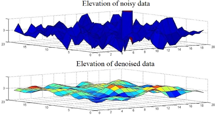
Many factors can affect the phase of the returned signal and make it unusable, such as the interaction with the surface factor. The phase of the wave may be deformed, depending on the properties of the material of the surface. Each pixel of the reflected signal is the summed contribution to the phase from many smaller targets in that ground area, each with different reflectivity properties and distances from the satellite; therefore, the effects of these factors must be eliminated in order to make the data usable. In order to remove these factors, interferometry uses a pair of images of the same area taken at slightly different positions and calculates the difference between their phases. Since the phase deforming factors have the same effect on both images, the difference between their phases eliminates these factors. The image that is created by this process is called an interferogram. In-SAR can also be used to calculate the third dimension similar to tomo-SAR [24]. Conventional In-SAR imaging systems usually use two-pass imaging with a little distance between the two tracks in order to cause a higher angle difference from the two images. Another form of In-SAR is to mount two SAR antennas on one platform, in which case it is a one-pass In-SAR [25]. Each of these methods has advantages and disadvantages over the other one. Both of these methods are demonstrated in Fig. 11. We have implemented In-SAR using Matlab; we have calculated the reflectivity and elevation of our dataset using this method. The resulted signals can be seen in Figs. 12 and 13.
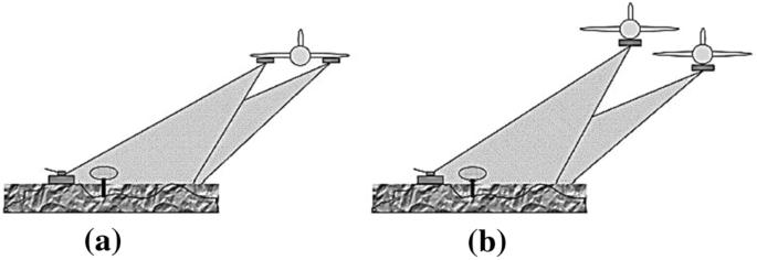
a One pass and b two pass SAR Interferometry
Reflectivity of the dataset \(500 \times 500\) estimated by In-SAR for noisy and denoised data
Elevation of the dataset \(20 \times 20\) pixels, estimated by In-SAR for noisy and denoised data
As it can be seen, this method produces acceptable results. The results of using denoised data are continues with much less singularities, meaning the algorithm has achieved answers for most pixels and that the noise in the elevation direction is sufficiently reduced. For this algorithm we have considered two scatterers in each cell.
6.4 Singular value decomposition
Singular Value Decomposition (SVD) is an important tool in linear algebra both as a decomposition and spectral estimation method. This method has many applications in signal processing and statistics. SVD of a rectangular matrix \(G_{M \times N}\) with \(M > N\), is a decomposition of the form of (13).
$$\begin{aligned} G=U \varSigma V^T=\varSigma u_i\cdot \sigma _i \cdot v_i^T ,\, for \, i=1,\ldots ,n \end{aligned}$$
(13)
In (13), \(U= (u_1 , \ldots , u_N )\) is the left singular vector or the eigenvector of \(G\cdot G^T\), \(V = (v_1 , \ldots , v_N )\) is the right singular vector or the eigonvector of \(G^T.G\) and \(\varSigma = diag(\delta _1, \ldots ,\delta _N)\) is a diagonal matrix holding the non-negative singular values of G [26]. The matrices generated through SVD are unique for a given matrix G. On of the applications of this method is in solving the spectrum estimation problem of tomo-SAR. The discrete reflectivity function \(\gamma\) can be reconstructed from \(\textit{g}\) through pseudo inversion of \(\textit{R}\) as in (14). Zhu et al. [23] combined this method with Wiener-type regularization to solve the tomo-SAR and differential tomo-SAR problems.
$$\begin{aligned} {\hat{\gamma }}=R^{\dagger } g = \sum _{n=1}^{N} \sigma _n ^{-1} (u_n^T \cdot g) \cdot v_n \end{aligned}$$
(14)
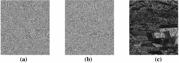
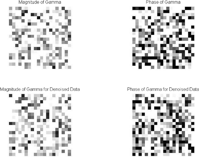
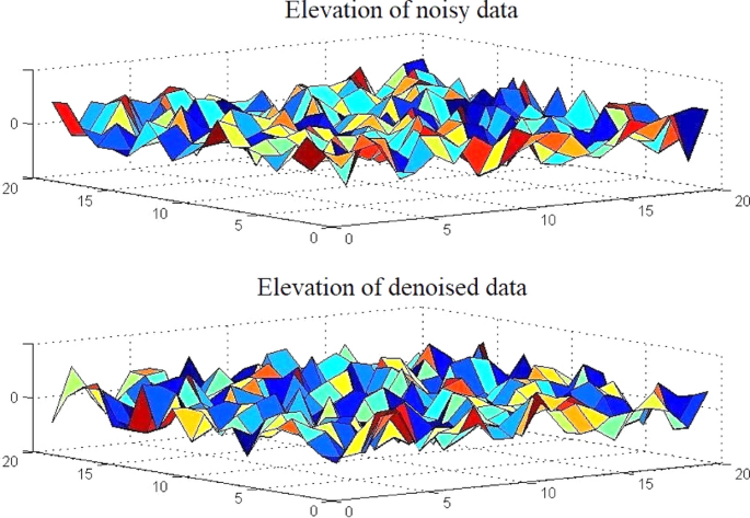
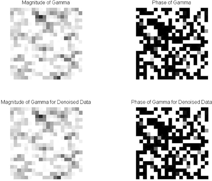
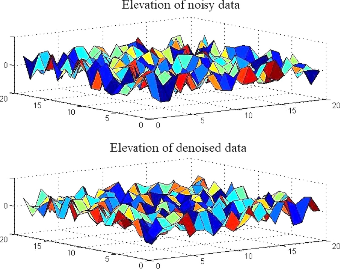
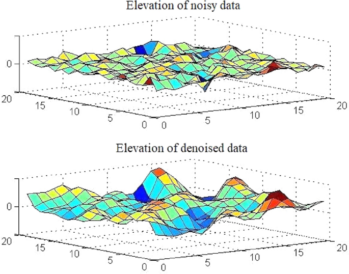
Although this method reaches acceptable results, the solution may include significant noise due to the nature of the problem. A well-known method to deal with the problem in (14) is the Truncated Singular Value Decomposition (TSVD). In this method extra requirements are forced in the solution, in order to reduce the error of (14). This process is done by discarding the components of the solution corresponding to the smallest singular values. Since this method resembles the Wiener filter with the white noise, the method is also named SVD-Wiener. This method is computationally efficient and is not sensitive to irregular sampling hence provides better results than conventional beamforming but not as good as NLS estimation. Figures 14 and 15 show the reflectivity and elevation of our dataset, calculated using this algorithm. We can see a significant difference between the elevation of noisy and denoised data. Elevation calculated from noisy data contains many singularities; however, for denoised data, all the spikes in the image which are indicators of singularity are gone. Therefore, although this method can achieve acceptable results, it is rather sensitive to the presence of noise.
Reflectivity of the dataset \(20 \times 20\) estimated by SVD
Elevation of the dataset \(20 \times 20\) estimated by SVD
6.5 Scale down by \(L_1\) norm minimization, model selection and estimation reconstruction
In Zhu and Bamler [27] first announced the possibility of using compressive sensing (CS) method in order to solve the SAR inversion problem and introduced the scale down by \(L_1\) norm Minimization, Model selection, and Estimation Reconstruction (SL1MMER) method, (pronounced “slimmer”). CS is a signal processing method that can reconstruct a signal from fewer measurements than what is specified in the Nyquist-Shannon sampling theorem by making use of certain characteristics of the certain signals [28]. The signal need to meet two conditions in order for CS to be able to reconstruct it. The first condition is sparsity, which means most of the signal’s samples must be zero and the second condition is for the signal to be incoherence and is met through the restricted isometry property (RIP) [29]. This is a relatively new subject in signal processing, and therefore, many of its applications are still not discovered [30]. Similar to the work of Zhu et al. [27], in Budillon and Schirinzi [31] developed a method to estimate the number of scatterers in each cell, using the same assumption of sparsity with support estimation and generalized likelihood ratio test (GLRT). There are also some preprocessing techniques in CS that can be employed in order to improve the quality of recovered signal, while sensing signal in smaller number of measurements [32]. The SLIMMER algorithm was initially developed for differential tomo-SAR (D-Tomo-SAR); however, it has been adapted and used for the tomo-SAR problem as well. The system of equations in (8)is severely underdetermined; Also the reflectivity function \(\gamma\) can be described as a sparse signal due to the following assumptions.
-
1.
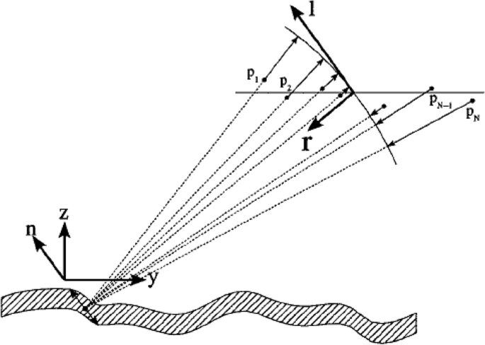
The scattered signal from completely vertical and horizontal surfaces is relatively weak; since they are not in the direction of the elevation, their contributions to the reflectivity is minimal. These weak reflections are shown in Fig. 16 with blue colors.
-
2.
Since most SAR imaging bands have the ability to penetrate the vegetation (except for bands that specialize in monitoring the vegetation), the scattered signal from these objects appears as noise, and their contributions are also minimal, as shown in Fig. 16 in green.
-
3.
The scattered signal from metallic objects or surfaces which are in the direction of the elevation (whether they are diagonal, or dihedral) is strong. These signals are shown in Fig. 16 in red.
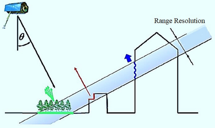
The effects of different scatteres on the tomo-SAR process within a resolution cell [33]
By using this logic, Zhu et al. assumed the reflectivity function to be sparse in the direction of elevation and used the CS method to solve this underdetermined problem [34, 35]. For achieving better results, the slimer algorithm also includes model order selection, which is added to the conventional algorithm. Considering the sparsity of the signal in elevation direction (\(K = 1 \sim 4\)), the reflectivity function \(\gamma\) can be very well defined using the \(l_0\)-norm minimization problem [36]. Similar minimization problems have been used in role determination approaches in order to identify the interaction modes in a haptic shared frameworks [37]. The sparsity of signal in the elevation direction is determined by the number of scatterers in each cell and the more numbers are considered the higher the computational complexity will be.
The \(l_0\)-norm minimization is an NP-hard problem; therefore one approach for solving it is to relax this equation into a \(l_1\)-norm minimization problem, this approach to solving the CS problem is known as basis pursuit (BP). In this study Zhu et al. estimated \(\gamma\) using the \(l_1\) and \(l_2\) norm minimization as is shown in (15).
$$\begin{aligned} {\hat{\gamma }}=arg\; min \{ \Vert g-R.\gamma \Vert _2^2 + \lambda _K\Vert \gamma \Vert _1 \} \end{aligned}$$
(15)
In (15) \(\Vert .\Vert\) shows the operator p-norm, and \(\lambda _K\) is a coefficient that is calculated based on the noise level [36]. CS shrinks \(\textit{R}\) considerably and gives a sparse estimation of the reflectivity function by only selecting columns corresponding to the non-zero elements of \(\gamma\); however since the measurement matrix is fixed and there are some violation of the RIP, this method would still would not be accurate enough by itself [38].
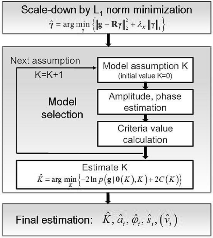
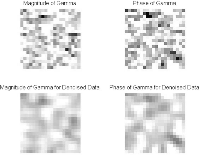
The three main phases of SLIMMER algorithm [9]
As it can be seen in Fig. 17, the next phase of this algorithm is model selection. In the previous phase, the size of \(\textit{R}\) is reduced, therefore, in this phase this algorithm tries to pinpoint the exact amount of \(\textit{K}\) by trying all the possible values of \(\textit{K}\) starting from one. Equation (16) describes the mathematical model of the model selection phase.
$$\begin{aligned} {\hat{K}}=arg\; min \{ -2\, ln \, p(g|{\hat{\theta }}(K),K)+2C(K) \} \end{aligned}$$
(16)
In (16), \(\theta (K)\) is defined as the vector holding the unknown variables of amplitude, phase and elevation for all scatterers, \(ln \, p(g|{\hat{\theta }}(K),K)\) is the log-likelihood of the observation model g with respect to the estimated \(\theta (K)\) and \(\textit{C(K)}\) is the complexity penalty; more information on each of these variables can be found in [23]. In each iteration, amplitude, phase, and elevation are estimated, and the error is calculated. In the last step, after \({\hat{K}}\) is calculated, the \(\textit{R}\) matrix will much slimmer than before (which is why this method is named SLIMMER). At this point, by using the new \(N \times {\hat{K}}\) measurement matrix, the reflectivity function and elevation are estimated. The sparse reflectivity function can be estimated using least square estimation equation of (11).
This method is computationally more efficient compared to NLS but is still expensive while the accuracy of this method is higher than SVD-Wiener. This process is not accurate enough to find the exact number of scatterers in each cell; instead, it limits the possibilities by setting an upper limit for the number of scatterers. We have applied this process to our dataset to find the number of scatterers. The \(l_1\)-minimization that we have implemented can calculate up to two scatterers in each cell which is sufficient for our dataset. The result of the first step of this method can be seen in Fig. 18 for an area of \(100 \times 100\) pixels. In Fig. 18 we can see a dark background with a few white dots. The dark pixels indicate the cells which have one scatterer while the white dots indicate cells that may have up to two to scatterers. In Fig. 18, the layover phenomenon can only occur in the white pixels and there are much fewer of them compared to the gray pixels. The scale-down part of the SLIMMER method can be combined with other methods as well. For example, we can scale down the sensing matrix by this technique and then use the SVD algorithm to estimate the elevation and reflectivity. This idea can open the door to many possibilities. In Liang et al. [39], took this idea further by assuming that the reflectivity is sparse not only in the direction of elevation but also range, making it a two-dimensional sparse signal and therefore can be retrieved using a two-dimensional CS recovery method. Similar to the work of Liang et al., We also published a paper in 2019 demonstrating that the reflectivity function is sparse in the range and azimuth plane. We further claimed that the reflectivity function is in fact a three-dimensional sparse signal [40].
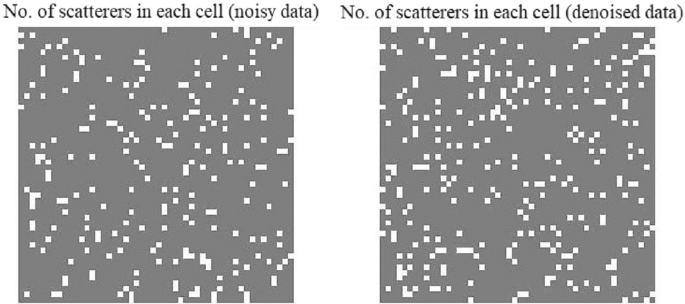
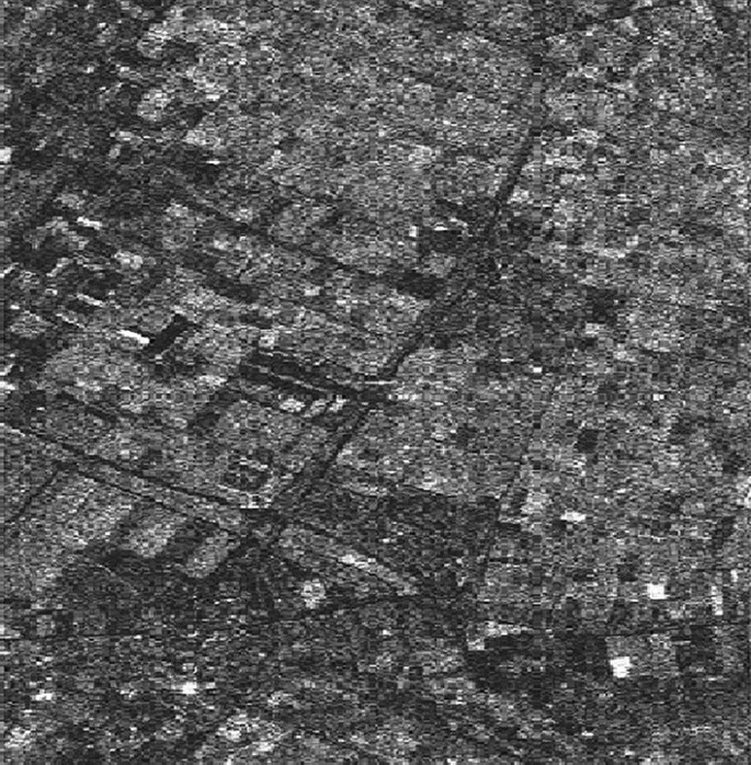
Number of scatterers in each cell of the dataset (the collected \(100 \times 100\)) for noisy and denoised data by \(L_1\)-minimization
7 Conclusion
SAR is a type of airborne radar which creates high resolution images by combining the physical aperture of the antenna with the aperture created by the movement of the radar over the scanned area. However, the acquired signals are only two-dimensional representation of the actual surface, and by losing the third dimension, much of real data would be lost. Aside from losing much of real data, losing the third dimension means that even the acquired two-dimension signal will not be accurate due to shadowing and layover phenomena. Tomo-SAR is the solution to this problem. By using several parallel acquisitions from the same area, it is possible to estimate the third dimension, which not only creates a more accurate model but also eliminates the shadowing and layover phenomena. Many estimation algorithms have been employed to calculate the third dimension. In this work, we chose five of the most used algorithms and explained each of them, both in theory and by using real data.
The beamforming method has a low computational time, but the results are not very accurate. The NLS estimation should have the best result theoretically; however, it has a very high computation time, which makes it impractical. In-SAR, as the predecessor of tomo-SAR, creates accurate models; especially if we take into consideration that this method only used two acquisitions. However, this method has a major flaw; it cannot detect different scatterers within each cell. SVD achieved the best estimation and had a smallest number of singularities between all the methods that were employed. The SLIMMER method also achieved accurate results and had better results regarding pixels with several scatterers; however, it is computationally more expensive than SVD. Therefore, using SLIMMER depends on the scanned area; for surfaces with many cells with multiple scatterers such as an urban environment or a mountain range, SLIMMER will have more accurate results and is more appropriate, even though it will have a higher computation time. As it was mentioned, scaling down the model using CS methods can be applied with other methods as well; also in for other CS methods besides BP might be helpful in the down scaling process. Creating a 3-dimensional sparse model can also potentially increase the accuracy of the estimations.
There are many other topics aside from spectral estimation related to this field that are being researched. Currently one of the popular topics in this area is using methods such as spatial regularization and non-local filtering to achieve high accuracy estimation of tom-SAR models with only few acquisitions (with few baselines) [41, 42]. Another area that has attracted many researchers in recent years is creating tomo-SAR models of vegetated areas such as forests [43, 44]. Tomo-SAR is still a developing technology and many of the topics related to it are still not discovered.
References
Ponce O, Prats-Iraola P, Scheiber R, Reigber A, Moreira A (2016) First airborne demonstration of holographic SAR tomography with fully polarimetric multicircular acquisitions at L-band. IEEE Trans Geosci Remote Sens 54(10):6170
Curlander JC, McDonough RN (1991) Synthetic aperture radar—systems and signal processing. Wiley, New York
Synthetic aperture radar. https://www.dlr.de/content/en/articles/missions-projects/terrasar-x/synthetic-aperture-radar.html. Accessed 17 June 2020
Minh DHT, Le Toan T, Rocca F, Tebaldini S, Villard L, Réjou-Méchain M, Phillips OL, Feldpausch TR, Dubois-Fernandez P, Scipal K et al (2016) SAR tomography for the retrieval of forest biomass and height: cross-validation at two tropical forest sites in French Guiana. Remote Sens Environ 175:138
Soumekh M (1999) Synthetic aperture radar signal processing, vol 7. Wiley, New York
Bamler R, Eineder M (2005) Accuracy of differential shift estimation by correlation and split-bandwidth interferometry for wideband and delta-k SAR systems. IEEE Geosci Remote Sens Lett 2(2):151
Fornaro G, Lombardini F, Serafino F (2005) Three-dimensional multipass SAR focusing: experiments with long-term spaceborne data. IEEE Geosci Remote Sens Lett 43(4):702
Budillon A, Johnsy AC, Schirinzi G (2017) A fast support detector for superresolution localization of multiple scatterers in SAR tomography. IEEE J Sel Top Appl Earth Observ Remote Sens 10(6):2768
Zhu XX, Bamler R (2011) Super-resolution power and robustness of compressive sensing for spectral estimation with application to spaceborne tomographic SAR. IEEE Trans Geosci Remote Sens 50:247
Pardini M, Papathanassiou K (2017) On the estimation of ground and volume polarimetric covariances in forest scenarios with SAR tomography. IEEE Trans Geosci Remote Sens Lett 14(10):1860
Budillon A, Evangelista A, Schirinzi G (2009) SAR tomography from sparse samples. In: 2009 IEEE international geoscience and remote sensing symposium, vol 4. IEEE, pp 4–865
Siddique MA, Wegmüller U, Hajnsek I, Frey O (2016) Single-look SAR tomography as an add-on to PSI for improved deformation analysis in urban areas. IEEE Trans Geosci Remote Sens 54(10):6119
Zink M, Bamler R (1995) X-SAR radiometric calibration and data quality. IEEE Trans Geosci Remote Sens 33(4):840
Tebaldini S, Nagler T, Rott H, Heilig A (2016) Imaging the internal structure of an alpine glacier via L-band airborne SAR tomography. IEEE Trans Geosci Remote Sens 54(12):7197
Lavalle M, Wright T (2009) Absolute radiometric and polarimetric calibration of ALOS PALSAR products. Document lssue (1), Revision (3)
Veci L (2015) TOPS Interferometry Tutorial. Sentinel-1 Toolbox
Plyer A, Colin-Koeniguer E, Weissgerber F (2015) A new coregistration algorithm for recent applications on urban SAR images. IEEE Geosci Remote Sens Lett 12(11):2198
De Zan F, Guarnieri AM (2006) TOPSAR: Terrain observation by progressive scans. IEEE Trans Geosci Remote Sens 44(9):2352
Esa sentinel level-1 product formatting. https://sentinel.esa.int/web/sentinel/technical-guides/sentinel-1-sar/products-algorithms/level-1-product-formatting. Accessed: 2020-06-01
Lombardini F, Reigber A (2003) Adaptive spectral estimation for multibaseline SAR tomography with airborne L-band data. In: IGARSS 2003. 2003 IEEE international geoscience and remote sensing symposium. Proceedings (IEEE Cat. No. 03CH37477), vol 3. IEEE, pp 2014–2016
Schmitt M, Stilla U (2014) Maximum-likelihood-based approach for single-pass synthetic aperture radar tomography over urban areas. IET Radar Sonar Navig 8(9):1145
del Campo Becerra GM, Nannini M, Reigber A (2018) Forest analysis using sar tomography and maximum likelihood inspired spectral estimation. In: EUSAR 2018. 12th European conference on synthetic aperture radar (VDE), pp 1–5
Zhu XX, Bamler R (2010) Very high resolution spaceborne SAR tomography in urban environment. IEEE Trans Geosci Remote Sens 48(12):4296
Adam N, Eineder M, Yague-Martinez N, Bamler R (2008) High resolution interferometric stacking with TerraSAR-X. In: IGARSS 2008–2008 IEEE international geoscience and remote sensing symposium, vol 2. IEEE, pp 2–117
Eineder M, Adam N, Bamler R, Yague-Martinez N, Breit H (2009) Spaceborne spotlight SAR interferometry with TerraSAR-X. IEEE Trans Geosci Remote Sens 47(5):1524
Strang G (1993) Introduction to linear algebra, vol 3. Wellesley-Cambridge Press, Wellesley, MA
Zhu X, Bamler R (2010) Super-resolution for 4-D SAR tomography via compressive sensing. In: 8th European conference on synthetic aperture radar (VDE), pp 1–4
Zhu XX, Bamler R (2014) Superresolving SAR tomography for multidimensional imaging of urban areas: compressive sensing-based TomoSAR inversion. IEEE Signal Process Mag 31(4):51
Li X, Liang L, Guo H, Huang Y (2015) Compressive sensing for multibaseline polarimetric SAR tomography of forested areas. IEEE Trans Geosci Remote Sens 54(1):153
Khoshnevis SA, Ghorshi S (2019) Recovery of event related potential signals using compressive sensing and kronecker technique. In: 7th IEEE global conference on signal and information processing (GlobalSIP), Ottawa, Canada
Budillon A, Schirinzi G (2015) GLRT based on support estimation for multiple scatterers detection in SAR tomography. IEEE J Sel Top Appl Earth Observ Remote Sens 9(3):1086
Mitra D, Zanddizari H, Rajan S (2019) Investigation of kronecker-based recovery of compressed ecg signal. IEEE Trans Instrum Meas 69(6):3642–3653
Zhu XX, Bamler R (2011) Sparse reconstrcution techniques for sar tomography. In: 2011 17th international conference on digital signal processing (DSP) (IEEE), pp 1–8
Zhu X (2011) Very high resolution tomographic sar inversion for urban infrastructure monitoring—a sparse and nonlinear tour. Ph.D. thesis, Technische Universität München
Zhu XX, Ge N, Shahzad M (2015) Joint sparsity in SAR tomography for urban mapping. IEEE J Sel Top Signal Process 9(8):1498
Zhu XX, Bamler R (2010) Tomographic SAR inversion by \(L_1\)-norm regularization—the compressive sensing approach. IEEE Trans Geosci Remote Sens 48(10):3839
Izadi V, Ghasemi A (2019) Determination of roles and interaction modes in a haptic shared control framework. In: Proceedings of the ASMA dynamic systems and control conference in Park City, Utah, pp 1–8
Montazeri S (2014) The fusion of sar tomography and stereo-sar for 3d absolute scatterer positioning. Master’s thesis, Delft University
Liang L, Li X, Ferro-Famil L, Guo H, Zhang L, Wu W (2018) Urban area tomography using a sparse representation based two-dimensional spectral analysis technique. Remote Sens 10(1):109
Khoshnevis SA, Ghorshi S (2019) Enhancement of the tomo-sar images based on compressive sensing method. In: 2019 6th international conference on space science and communication (IconSpace). IEEE, pp 41–46
Rambour C, Denis L, Tupin F, Oriot HM (2019) Introducing spatial regularization in SAR tomography reconstruction. IEEE Trans Geosci Remote Sens 57(11):8600
Shi Y, Bamler R, Wang Y, Zhu XX (2020) SAR tomography at the limit: building height reconstruction using only 3–5 TanDEM-X Bistatic Interferograms. arXiv preprint arXiv:2003.07803
El Moussawi I, Ho Tong Minh D, Baghdadi N, Abdallah C, Jomaah J, Strauss O, Lavalle M, Ngo YN (2019) Monitoring tropical forest structure using SAR tomography at L-and P-Band. Remote Sens 11(16):1934
d’Alessandro MM, Tebaldini S (2019) Digital terrain model retrieval in tropical forests through P-band SAR tomography. IEEE Trans Geosci Remote Sens 57(9):6774


No comments:
Post a Comment